Statistical Mechanics
Large Numbers
Intensive: \(O(N^0) = O(1)\).
Extensive: \(O(N^1) = O(N)\). Note: Ext/Ext = Int, Int x Ext = Ext.
Exponentially Large: \(O(e^N)\).
How many microstates in a simple system. Consider a site with 2 states or a 4x4 grid, \(N=N_s^2=4^2=16\).
Ising model, \(s_i=\{-1,+1\}\).
In the 4x4 grid, we have \(2^{16}=65536\) states. An exaflop is \(10^{18}\) floating point operations per second which is roughly \(2^{60}\).
Estimate, 1000 Exaflops total in the world, \(2^{10}\).
30 million seconds, \(3\cdot10^7\). Then, \(2^25\). So, \(2^{95}\) sites can be calculated in a year. If we double in a year, we can calculate one more site.
Roughly, \(2^{80}\) atoms in the universe.
\(S = \sum_\alpha \exp\left(\frac{E_\alpha}{kT}\right)\), \(E_\alpha = \sum_{i=1}^N\epsilon_i\).
\(S = \sum_{\alpha=1}^{N^P}Y_\alpha\), \(0\leq Y_\alpha \sim O(\exp(N\phi_\alpha))\). We can choose it to be bounded below by any number we choose, but zero is typically most convenient. Then, \(0\leq Y_\alpha\leq Y_max\).
So, \(y_{max}\leq S\leq N^{P}y_{max}\).
Consider, \(\frac{\ln S}{N}\). Then, \(\frac{\ln y_{max}}{N}\leq \frac{\ln S}{N} \leq \frac{p\ln N}{N} + \frac{\ln y_{max}}{N}\). As \(N\to\infty\), \(\ln N/N\to 0\), so \(\frac{\ln S}{N}\approx \frac{\ln y_{max}}{N}\), hence \(\ln S\approx \ln y_{max}\).
Integrals
\(I = \int dx \exp(N\phi(x))\). Approximating these by the maximum value of integrand (φ(xmax)) obtained at \(x=x_{max}\).
Taylor expanding around this point, \(J\approx \int dx \exp \left(N\left(\phi(x_{max}) + \frac{1}{2}\phi(x-x_{max})^2+\cdots\right)\right)\). \(\phi'(x_{max}) = 0, \phi''(x_{max})<0\) due to \(x\) being a maxiumum.
\(J\approx\exp(N\phi(x_{max}))\int dx\exp \left(-\frac{N}{2}|\phi''(x_{max})|(x-x_{max})^2\right) = \sqrt{\frac{2\pi}{N/\phi''(x_{max})}}\exp(N\phi(x_{max}))\).
2 major corrections are needed:
- Higher order terms: powers of 1/N
- Other local maxima: xmax’ will have a different size (Assumed a single maximum, but there may be other maximums as well as higher or lower maximums.) The relative size goes to zero as \(N\to\infty\), \(\frac{\exp(N\phi(x'))}{\exp(N\phi(x))} = \exp(-N(\phi(x)-\phi(x')))\) has a positive inner argument and an overall minus sign.
Write \(\phi(x) = \ln x - \frac{x}{N}\). Then, \(\int_0^\infty \exp(N\phi(x)) dx = \int_0^\infty x^N\exp(-x)dx = \Gamma(N+1)\). \(\phi_max = \phi'(x) = \frac{1}{x} - \frac{1}{N}\). Then the maximum is at \(x=N\). \(\phi(x_{max}) = \ln N-1\). \(\phi''(x) = -\frac{1}{x^2}\to \phi''(x_{max}) = -\frac{1}{N^2}\). So, \(N!=\int_0^\infty x^N\exp(-x)\approx \exp(N\phi(x_{max}))\int dx \exp \left(-\frac{N}{2}|\phi''(x_{max})|(x-x_{max})^2\right) = \frac{N^N}{e^N}\sqrt{2\pi N}\).
Gamma Function
\(\int dx x^n\exp(-x) = \Gamma(n+1) = n!\).
Partition Function
\(Z = \sum_\alpha\exp(-\beta E_\alpha)\). \(p_\alpha = \frac{\exp(-E_\alpha/kT)}{Z}\).
\(\langle E\rangle = \sum_\alpha p_\alpha E_\alpha = -\frac{1}{Z}\partial_\beta Z = -\frac{\partial\ln Z}{\partial\beta}\).
\(\frac{\partial\langle E\rangle}{\partial T} = \frac{\partial \langle E\rangle}{\partial \beta}\frac{\partial \beta}{\partial T}\)
C.f. \(C_V = \left(\frac{\partial U}{\partial T}\right)_{V,N}\)
\(C_v = f(\langle E\rangle, \langle E^2\rangle) = \gamma(\langle E^2\rangle - \langle E\rangle^2)\).
Disorder
Entropy of Mixing
Consider a system with two parts of equal volume, \(V\). Total volume \(2V\). \(N\) total particles. Put the particles equally distributed in both regions, \(N/2\). Color the left white and the right black. The entropy for the right or left atoms is then, \(S_{W,B} = k_B\ln \frac{V^{N/2}}{\left(\frac{N}{2}\right)!}\).
\(\Omega(E) = \left(\frac{V^N}{N!}\right)\left(\frac{(2\pi mE)^{\frac{3N}{2}}}{\left(\frac{3N}{2}\right)! h^{3N}}\right)\) = space * momentum.
\(S_{unmixed} = 2S_{W,B} = 2k_B\ln\frac{V^{N/2}}{(N/2)!}\) \(S_{mixed} = 2(k_B\ln\frac{(2V)^{N/2}}{(N/2)!})\). \(\Delta S_{mixing} = S_{mixed} - S_{unmixed} = 2k_B\ln\left(\frac{(2V)^{N/2}}{V^{N/2}}\right) = Nk_B\ln 2\).
Gibbs Paradox
If the particles were both black. \(S_{unmixed} = 2S_{W,B} = 2k_B\ln\frac{V^{N/2}}{(N/2)!}\) \(S_{mixed} = k_B\ln\frac{(2V)^{N}}{N!}\). \(\Delta S_{mixing} = S_{mixed} - S_{unmixed} = k_B\ln\left(\frac{2^N\left(\frac{N}{2}\right)!^2}{N!}\right)\). Using the Stirling approximation, \(\Delta S_{mixing}/k_B = N\ln 2 + 2\left(\frac{N}{2}\ln\frac{N}{2}-\frac{N}{2}\right)-(N\ln N-N) = N\ln N - N - N\ln 2 + N\ln 2- (N\ln N-N) = 0\).
Materials
Amorphous Solids
Glasses
The Solids are glasses if they have a glass transition.
If you heat up to a temperature \(T\) then cool slowly, as you cool you phase transition between liquid and crystal solid at \(T_{melt}\).
If you do it quickly to a temperature below \(T_{glass}
In order to redo a glass, you have to go back above \(T_{melt}\) and recool to \(T_g\).
You get a unit of entropy (kB) per unit of material.
Theoretical glass models:
- Spin-glasses. Consider a lattice of sites with spins \(\pm 1\). Say we have some random interaction \(Js_is_j\). If \(J\) is positive, then you need a even number of neighbors to get a non-frustrated glass. I.e. if you have a hexagonal lattice you get frustration. \(- slow -> Crystal - slow -> Liquid - fast -> Glass\) \(S_{res} = S_\ell(T_\ell) - \int \frac{1}{T}\frac{dQ}{dt}dt = S_\ell(T_\ell) - \int_0^{T_\ell}\frac{1}{T}\frac{dQ}{dT}dT \propto k_B\times \#\text{molecular units}\). Remark: \(\frac{dQ}{dT}\) is the heat capacity.
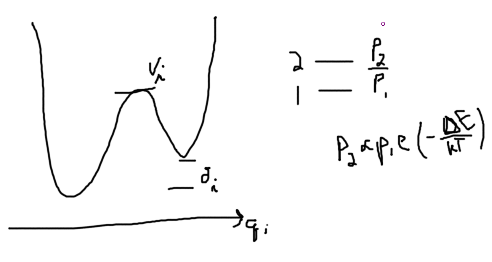
Assuming, \(V_i\gg \delta_i\). If kinetics is important minimal will be occupied roughly equally, \(\Delta S_{q_i} = k_B\ln 2\). [then when you cool from the high temperature state (assuming \(V_i\gg \delta_i\)), you will find that some of the \(2\) states will remain since they cannot traverse the barrier to get to the one state.]
The energy stored in the higher state by accident is \(\delta_i\) per \(q_i\), (50%). \(\Delta S_{q_i} \sim \frac{\Delta Q_i}{T}\). Note, we only have two temperatures, \(T_1 \sim \frac{V_i}{k_B}\) and \(T_2 \sim \frac{\delta_i}{k_B}\ll\frac{V_i}{k_B}\). In our case, \(T=T_2\). We can call \(T\), \(T_{freeze}\). So, \(T_{freeze} \sim \frac{\delta_i}{k_B}\ll\frac{V_i}{k_B} \sim \frac{\delta_i}{\frac{\delta_i}{k_B}}\sim k_B\).
The time scale for this hopping is \(\tau\sim 10^{-12}\) s.
Lenard-Jones potential - Annealing MC - 39 particles. Numerical does not give good results. Can only solve the system classically and then simulate the dynamics for reasonable results.
Information Theory
Initial Remarks
If you cannot get or use the information then the entropy does not change for a system. (The information to be put in the next process)
The information you can gain about the system. It is external to the system but is a state variable.
Lecture
\(S_{discrete} = -k_B\langle\ln p_i\rangle = -k_B\sum_i p_i\ln p_i = -k_B\sum_i\frac{1}{W}\ln\frac{1}{W} = k_B \ln W = k_B\int_{E<\mathcal{H}(\mathbb{P},\mathbb{Q}) < E+\delta E}\frac{d\mathbb{P}d\mathbb{Q}}{\delta N}\rho(\mathbb{P},\mathbb{Q})\ln\rho(\mathbb{P},\mathbb{Q}) = -k_B\text{Tr}(\hat{\rho}\ln\hat{\rho})\) with \(\rho:=\) density matrix. Some texts call \(\langle \ln p\rangle\) the suprisal fuction, the ensemble average of ’suprise’.
Examples
Box: 3 balls: 1 red, 2 green.
For the first draw: \(p(R) = \frac{1}{3}, p(G) = \frac{2}{3}\).
If we put it back, we get independent draws. For the second draw (without putting back): \(p(R_2) = p(R_1)p(R_2|R_1) + p(G_1)p(R_2|G_1) = 0 + \frac{2}{3}1 = \frac{1}{3}\), \(p(G_2) = p(R_1)p(G_2|R_1) + p(G_1)p(G_2|G_1) = \frac{1}{3}(1) + \frac{2}{3}\frac{1}{2} = \frac{2}{3}\).
For the third draw (without putting back): \(p(R_3) = p(G_1G_2)p(R_3|G_1G_2) = p(G_1)p(G_2|G_1)p(R_3|G_1G_2) = \frac{2}{3}\frac{1}{2} = \frac{1}{3}\). \(p(G_3) = 1-p(R_3) = \frac{2}{3}\).
Measure of Suprise
What is information…
You won the Lottery! -> Huge suprise because it is highly unlikely. I.e. \(p\to 0\). So suprise \(\to\infty\).
You didn’t win the Lottery! -> ’Almost’ no suprise since it is highly likely. I.e. \(p\to 1\) so suprise \(\to 0\).
Note, \(-\ln p\) has this behavior.
Information
Notation: outcomes \(A_k;k=1,\cdots,\Omega;p_k=p(A_k);\sum_k p_k=1;B_\ell,\ell=1,\cdots,M;q_\ell=p(B_\ell);\sum_\ell q_\ell=1\). For instance, if \(A_k\) are the possible location for your keys and \(B_\ell\) are the locations that you last saw the keys.
- Information is max if all the outcomes are equally likely. \(S_I\left(\frac{1}{\Omega},\cdots,\frac{1}{\Omega}\right)\geq S_I(p_1,\cdots,p_\Omega)\) with equality only if \(p_i=\frac{1}{\Omega}\forall i\).
- Information does not change if we add outcomes \(A_j\) with \(p_j=0\). \(S_I(p_1,\cdots,p_{\Omega-1}) = s_I(p_1,\cdots,p_{\Omega-1},0)\).
- If we obtained (measure) partial information for a joint outcome \(C=A\cdot B\) by measuring \(B\) then \(\langle S_I(A|B_\ell)\rangle_B = S_I(C)-S_I(B)\) where \(\langle S_I(A|B_\ell)\rangle_B = \sum_{\ell=1}^M S_I(A|B_\ell) q_\ell\). Note, \(C_{k\ell} = A_k\cdot B_\ell, r_{k\ell} = p(C_{k\ell})\). We use the average since we don’t know the answer a priori and so we must consider all of the possibilities. Once we have a specific \(B_\ell\) then that \(q_\ell=1\) and the rest are zero, and so this still holds up.
\(C_{k\ell} = P(A_k|B_\ell) = \frac{P(B_\ell|A_k)P(A_k)}{P(B_\ell)} = \frac{P(A_k\wedge B_\ell)}{p(B_\ell)} = \frac{P(A_kB_\ell)}{p(B_\ell)} = \frac{r_{kl}}{q_\ell}\).
\(\sum_k c_{k\ell} = \sum_k P(A_k|B_\ell) = 1\).
Before you talk to your roommate, \(S_I(A\cdot B) = S_I(r_{11},r_{12},\cdots,r_{1M},r_{21},\cdots,r_{\Omega,M}) = S_I(c_{11}q_1,c_{12}q_2,\cdots,c_{\Omega M}q_M)\).
After you talked to your roomate, \(S_I(A|B_\ell)\). % = S(r1ℓ,r2ℓ,⋯,rΩℓ) Expected change in \(S_I\) if you measure is given by (rule 3) \(\langle S_I(A|B_\ell)\rangle_B = S_I(C) - S_I(B) = \sum_{\ell=1}^m S_I(A|B_\ell)q_\ell\).
Proving 3. \(S_I(C) = S_I(AB) = -k_S\sum_{k\ell}r_{k\ell}\ln r_{k\ell} = -k_S\sum_{k\ell}c_{k\ell}q_\ell\ln(c_{k\ell}q_\ell) = -k_S\left[\sum_{k\ell}c_{k\ell}q_\ell\ln c_{k\ell} + \sum_{k\ell}c_{k\ell}q_\ell\ln q_\ell\right] = \sum_\ell q_\ell(-k_S\sum_k c_{k\ell}\ln c_{k\ell}) - k_S\sum_\ell\left[q_\ell \ln(q_\ell)\sum_k c_{k\ell}\right] = \sum_\ell q_\ell(-k_S\sum_k c_{k\ell}\ln c_{k\ell}) - k_S\sum_\ell\left[q_\ell \ln(q_\ell)\right] = \sum_{\ell}q_\ell S_I(A|B) + S_I(B) = \langle S_I(A|B_\ell)\rangle_B + S_I(B)\).
Proving 2. \(S_I = -k_S\sum_k^\Omega p_k\ln p_k = -k_S\sum_k^{\Omega-1}p_k\ln p_k + \lim_{p\to 0}p\ln p = S_I^{\Omega-1}\).
Proving 1. \(f(p) = -p\ln p\). Thus, it is the information for 1 variable. \(\frac{df}{dp} = -\ln p-1\). \(\frac{d^2f}{dp^2} = -\frac{1}{p} < 0\) for \(p\in(0,1)\). Thus, \(f(p)\) is concave.
For any points \(a,b\) the weighted average \(\lambda a+(1-\lambda) b\). Then,
\begin{equation}\tag{x} (\lambda a+(1-\lambda)b)\geq\lambda f(a) + (1-\lambda)f(b). \end{equation}Jensen inequality. \(f\left(\frac{1}{\Omega}\sum_k p_k\right) \geq \frac{1}{\Omega}\sum_k f(p_k)\).
Consider \(\Omega = 2\). In \((x)\) choose \(\lambda = \frac{1}{2}\), \(a=p_1,b=p_2\). Then, \(f\left(\frac{p_1+p_2}{2}\right) \geq \frac{1}{2}(f(p_1)+f(p_2))\).
For a general \(\Omega\), choose \(\lambda = \frac{\Omega-1}{\Omega}\), \(a=\frac{1}{\Omega-1}\sum_k p_k\) and \(b=p_\Omega\). Then by induction on \(a\) and including \(b\) with the \(\Omega=2\), we get the result we want. So, \(f\left(\frac{1}{\Omega}\sum_k p_k\right) = f\left(\frac{\Omega-1}{\Omega}\sum_k^{\Omega-1}\frac{p_k}{\Omega-1}+\frac{1}{\Omega}p_\Omega\right) \geq \frac{\Omega-1}{\Omega}f\left(\sum_k^{\Omega-1}\frac{p_k}{\Omega-1}\right) + \frac{1}{\Omega}f(p_\Omega)\) Assuming the Jensen inequality is true, \(f\left(\frac{1}{\Omega}\sum_k p_k\right) = f\left(\frac{\Omega-1}{\Omega}\sum_k^{\Omega-1}\frac{p_k}{\Omega-1}+\frac{1}{\Omega}p_\Omega\right) \geq \frac{\Omega-1}{\Omega}f\left(\sum_k^{\Omega-1}\frac{p_k}{\Omega-1}\right) + \frac{1}{\Omega}f(p_\Omega) \geq \frac{1}{\Omega}\sum_k^{\Omega-1}f(p_k)+\frac{1}{\Omega}f(p_\Omega) = \frac{1}{\Omega}\sum_k f(p_k)\).
So, \(S_I(p_1,\cdots,p_\Omega) = -k_S\sum_k p_k\ln p_k = k_S \sum_k f(p_k) = k_S\Omega \frac{1}{\Omega}\sum_k f(p_k) \leq k_S\Omega f\left(\frac{1}{\Omega}\sum_k p_k\right) = k_S\Omega f\left(\frac{1}{\Omega}\right) = -k_S\Omega\frac{1}{\Omega}\ln\frac{1}{\Omega} = -k_S \ln\frac{1}{\Omega} = S_I\left(\frac{1}{\Omega},\cdots,\frac{1}{\Omega}\right)\).
Conditional Probability
Definition: \(p(B|A)\) is probability of event \(B\) given event \(A\) was observed.
Joint
\(p(A\wedge B) = p(AB)\).
Bayes Rule
\(p(AB) = p(B|A)p(A) = p(A|B)p(B)\).
Independent
For independent events, \(p(B|A) = p(B)\), \(p(A|B) = p(A)\). So, \(p(AB) = p(A)p(B)\).
Beyond the Microcanonical Ensemble
Information Theory Approach
Maximize entropy, minimize bias, principle.
Max: \(S=-k_B\sum_\alpha p_\alpha\ln p_\alpha\) subject to constraints using Lagrange parameters.
Constraints:
- \(\sum_\alpha p_\alpha = 1\)
- \(\langle E\rangle = \sum_\alpha p_\alpha E_\alpha \equiv E\equiv U\)
If you do just (1), then you get \(p_\alpha = \frac{1}{N_\alpha}\).
If you do both (1+2), then \(\mathcal{L} = -k_B\sum_\alpha p_\alpha\ln p_\alpha + \lambda_1 k_B(1-\sum_\alpha p_\alpha)+\lambda_2 k_B(U-\sum_\alpha p_\alpha E_\alpha)\).
\(\frac{\partial\mathcal{L}}{\partial p_\alpha} = \cdots = 0\)
How does the temperature enter?
\(\lambda_2 = \beta = \frac{1}{k_BT}\).
From the Microcanonical Ensemble
Recall we had the partitioned volume with sides at \(S_1,E_1,\rho(E_1)\) and \(E-E_1\) with \(\rho(S_1) = \frac{\Omega_2(E-E_1)}{\Omega(E)}\).
\(\rho(E_1) = \frac{\Omega_1(E_1)\Omega_2(E-E_1)}{\Omega(E)}\). Maximize \(\rho(E_1)\) leads to \(\frac{1}{\Omega_1}\left(\frac{\text{d} \Omega_1}{\text{d} E_1}\right)_{E_1^*}= \frac{1}{\Omega_2}\left(\frac{\text{d} \Omega_2}{\text{d} E_2}\right)_{E-E_1*}\)
Define \(S\): \(\left(\frac{dS_1}{dE_1}\right)_{E_1^*,V_1,N_1} = \left(\frac{dS_2}{dE_2}\right)_{E-E_1^*,V_2,N_2}\)
Define \(T\) \(\frac{1}{T_1} = \frac{1}{T_2}\).
If we consider 1 as the system and 2 as the heat bath/ environment, So, \(\rho(S) = \frac{\Omega_2(E-E_S)}{\Omega(E)} = \frac{1}{\Omega(E)}\exp\left(\frac{S_2(E-E_S)}{k_B}\right)\).
Comparing two states, \(S_A, E_A\) and \(S_B, E_B\). Assume \(E_B>E_A\), but this is not required.
\(\frac{\rho(S_B)}{\rho(S_A)} = \frac{\Omega_2(E-E_B)}{\Omega_2(E-E_A)} = \exp\left(\frac{S_2(E-E_B)-S_2(E-E_A)}{k_B}\right)\)
Note, \(S_2(E-B_B) - S_2(E-E_A)\approx (E_A-E_B)\left(\frac{\partial S}{\partial E}\right)\)
This comes from \(\Delta S_2 = \frac{\Delta E_2}{T}\). So, \(\Delta E_{sys} = \Delta E_1=E_B-E_A\). So, \(\Delta E_{env} = -\Delta E_{sys} = E_A-E_B\).
Then, probability in being in a particular state is \(\rho(S) \propto \exp\left(-\frac{E_S}{k_BT}\right) = \exp(-\beta E_S)\).
Normalization: \(sum_\alpha \rho(S_\alpha) = 1\Rightarrow \rho(S) = \frac{\exp(-\beta E_S)}{\sum_\alpha\exp(-\beta E_\alpha)} = \frac{1}{Z}\exp(-\beta E_S)\).
\(Z = \sum_\alpha\exp(-\beta E_\alpha) = \int\frac{d\mathbb{P}_1\mathbb{Q}_1}{h^{3N_1}}\exp\left(-\frac{H_1(\mathbb{P}_1,\mathbb{Q}_1)}{kT}\right) = \int dE_1\Omega_1(E_1)\exp\left(-\frac{E_1}{kT}\right)\).
Internal energy: \(\langle E\rangle = \sum_\alpha p_\alpha E_\alpha = \frac{1}{Z}\sum_\alpha E_\alpha\exp(-\beta E_\alpha) = -\frac{\partial\ln Z}{\partial B}\).
Heat capacity at a constant volume: \(c_V = \left(\frac{\partial U}{\partial T}\right)_{V,N} = \left(\frac{\partial \langle E\rangle}{\partial T}\right) = \frac{\partial\langle E\rangle}{\partial\beta}\frac{\partial\beta}{\partial T} = -\frac{1}{k_BT^2}\frac{\partial\langle E\rangle}{\partial\beta} = \frac{1}{k_BT^2}\frac{\partial^2\ln Z}{\partial\beta^2}\). \(c_V = T\left(\frac{\partial S}{\partial T}\right)_{V}\).
\(\frac{\partial\langle E\rangle}{\partial \beta} = -\frac{\partial}{\partial\beta}\frac{\sum_\alpha E_\alpha\exp(-\beta E_\alpha)}{\sum_\alpha\exp(-\beta E_\alpha)} = \frac{1}{Z^2}\left(\sum_\alpha (-E_\alpha)\exp(-\beta E_\alpha)\right)\left(\sum_\alpha E_\alpha\exp(-\beta E_\alpha)\right) + \frac{1}{Z}\sum_\alpha E_\alpha^2\exp(-\beta E_\alpha) = -\langle E\rangle^2 + \langle E^2\rangle = \langle(E-\langle E\rangle)^2\rangle = \langle E^2 -2E\langle E\rangle+\langle E\rangle^2\rangle = \langle E^2\rangle - \langle E\rangle^2\).
The total heat capacity is then \(C_V = N\tilde{c}_V = \frac{1}{k_BT^2}(\langle E^2\rangle - \langle E\rangle^2) = \frac{\sigma_E^2}{k_BT^2}\).
The energy fluctuations per particle is \(\frac{\sigma_E}{N} = \frac{\sqrt{\langle E^2\rangle-\langle E\rangle^2}}{N} = \frac{\sqrt{N\tilde{c}_Vk_BT^2}}{N} = \frac{\sqrt{k_BT}\sqrt{\tilde{c}_VT}}{\sqrt{N}}\). The second square root is related to the amount of heat required to rais individual particle temperatures.
So, for large systems the energy fluctuations per particle remain small. So you can analyze the system cannonically or microcannonically.
\(S = -k_B\sum_\alpha p_\alpha\ln p_\alpha = -k_B\sum_\alpha\frac{\exp(-\beta E_\alpha)}{Z}\ln\left(\frac{\exp(-\beta E_\alpha)}{Z}\right) = -k_B\frac{1}{Z}\sum_\alpha\left(\exp(-\beta E_\alpha)\ln(-\beta E_\alpha-\ln Z)\right) = k_B\beta\langle E\rangle + k_B\ln Z\sum_\alpha\frac{\exp(-\beta E_\alpha)}{Z} = k_B\ln Z + \frac{\langle E\rangle}{T}\). So, \(-k_BT\ln Z = \langle E\rangle-TS=U-TS = F\).
Thus, we get the Helmholtz free energy from the partition function.
Equivalently, \(Z = \exp(-\beta F)\).
So, connecting a system to a heat bath is the most basic assumption we need to derive our thermodynamic quantities we are familiar with.
Exercise
We have, \(Z = \exp(-\beta E) = \exp(-\beta H)\). Consider a conjugate pair, \(X,y\) (i.e. y is a generalized force and X is a generalized displacement), then \(\mathcal{X} = \frac{\partial X}{\partial y}\). We then get \(Z=\exp(-\beta(H-Xy))\). So, \(E=E(X)\) for internal energy.
Quantum Statistical Mechanics
\(N(\mu) = \int_0^\infty d\epsilon g(\epsilon)n(\mu, T)d\epsilon\).
For 3D: \(g(\epsilon) = (4\pi p^2) \left(\frac{d|\vec{p}|}{d\epsilon}\right)\left(\frac{L}{(2\pi\hbar)}\right)^3\). For 2D: \(g(\epsilon) = (2\pi p) \left(\frac{d|\vec{p}|}{d\epsilon}\right)\left(\frac{L}{(2\pi\hbar)}\right)^2\). For 1D: \(g(\epsilon) = (2) \left(\frac{d|\vec{p}|}{d\epsilon}\right)\left(\frac{L}{(2\pi\hbar)}\right)^1\).
Thermal Equilibrium
Particles in thermal equilibrium follow a boltzman distribution.
Nucleation
We are reaching for droplet formation from gas to liquid abrupt phase transition.
\(\Delta G = G_{gas} - G_{liquid}\) Dividing across by \(N\), \(\Delta \mu = \frac{\Delta G}{N} = \frac{G_{gas} - G_{liquid}}{N}\).
\(\Delta G\approx \frac{\partial(G_{g}-G_{\ell})}{\partial T}\Delta T = (S_{\ell}-S_{g})\Delta T\) So, \(\Delta\mu\approx \frac{(S_{\ell}-S_g)\Delta T}{N}\). And, \(\Delta S_{L-G} = \frac{Q}{T_v} = \frac{L\cdot N}{T_v}\). So, \(\Delta\mu = \frac{L\Delta T}{T_v}\).
Consider a droplet of volume \(V_D\). Then, \(\Delta G\propto V_D\) which lowers the free energy. The surface costs energy: \(\propto \sigma A_D\) where \(\sigma\) is the surface tension and raises the free energy.
\(\Delta G = 4\pi R^2\sigma - \frac{4}{3}\pi R^3\frac{N\Delta\mu}{V} = 4\pi R^2\sigma - \frac{4}{3}\pi R^3 n\Delta\mu\). Then, we get some critical radius, \(R_c\) between these two competing free energies. \(R_c = \frac{2\sigma}{n\Delta\mu} = \frac{2\sigma T_v}{nL\Delta T}\) gives the critical radius of the droplet. Hence, for lower barriers (lower latent heat) the critical radius increases. The barrier, \(B = \frac{16\pi \sigma^3 T_v^2}{3n^2 L^2(\Delta T)^2}\).
Conserved order parameter: (mass) requires conservation of quantities. Non-conserved order parameter: (magnetism).
Introduction to Phenomonological Scaling
- \(\alpha\): \(C_\beta\propto \left|\frac{T-T_c}{T}\right|^{-\alpha}\) where \(T\to T_c\) and \(B=0\).
- \(\beta\): \(m\propto (T_c-T)^\beta\) where \(T\to T_c\), \(T>T_c\), and \(B=0\)
- \(\gamma\): \(\chi\propto |T_c-T|^{-\gamma}\) where \(T\to T_c\) and \(B=0\)
- \(\delta\): \(m\propto B^{1/\delta}\) where \(T= T_c\) and \(B=0\)
- \(\eta\): \(C_c^{(2)}(r)\ propto \frac{1}{r^{d-2+\eta}}\) where \(T=T_c\) and \(B=0\)
- \(\nu\): \(C_c^{(2)}(r)\propto\exp(-r/\xi)\) and \(\xi\propto|T-T_c|^{-\nu}\) for \(B=0\) and \(T\) near \(T_c\)
Widom Scaling Hypothesis. The free energy, \(f(T,B) = t^{1/y}\psi\left(\frac{B}{t^{x/y}}\right)\) where \(t = \frac{|T-T_c|}{T_c}\). So, \(z = \frac{B}{t^{x/y}}\to t^{x/y} = \frac{1}{z}\frac{B}{z} \Leftrightarrow t^{1/y} = \frac{B^{1/x}}{z^{1/x}}\). So, \(f(T,B) = B^{1/x}z^{-1/x}\Psi(z) = B^{1/x}\tilde{\psi}\left(\frac{B}{t^{x/y}}\right)\). Then, \(m_{B=0} = -\left(\frac{\partial f}{\partial B}\right)_T = -t^{(1-x)/y}\psi'(0)\) and \(\beta = \frac{1-x}{y}\). From this, we can calculate the first 4, which come in combinations of \(x\) and \(y\). For \(\chi\), \(\gamma = \frac{2x-1}{y}\). For \(C_B\), \(\alpha = 2 - \frac{1}{y}\). Also, \(\delta = \frac{1}{x}-1\).
Hausdorf Scaling Hypothesis, \(C_c^{(2)}(r, t) = \frac{\psi(r t^{\frac{2-\alpha}{d}})}{r^{d-2+\eta}}\). So, \(\gamma d=\alpha-2\). From all of these, we see that 5-6 only depend on 2 parameters needed.