Quantum Statistical Mechanics
QMHO
\(\hat{H} = \frac{\hat{p}^2}{2m} + \frac{m\omega^2 x^2}{2} = \hbar\omega(b^\dagger b+1/2)\) with energies \(E_n = \left(n+\frac{1}{2}\right)\hbar\omega\).
\(Z_{QHO} = \sum_n \exp(-\beta E_n)\).
\(\langle E\rangle_{QHO} = \hbar\omega\left(\frac{1}{2} + \frac{1}{\exp(\beta\hbar\omega) - 1}\right)\) with \(\langle n\rangle = \frac{1}{\exp(\beta\hbar\omega)-1}\) - which looks like \(\langle n\rangle_{BE}\) with \(\mu=0\). BE is Bose-Einstein, \(E(k) = \frac{\hbar^2k^2}{2m}\). We set \(\mu=0\) since we can add or remove particles freely to this bosonic state without affecting the other particles.
Consider if we have an energy of \(\hbar\omega\) and we populate it with \(n\) particles, then we get the same \(\hat{H} = \hbar\omega(b^\dagger b + 1/2) = \hbar\omega(n+1/2)\). Thus, we can consider a \(n-\) energy level a bosonic gas of \(n\) particles with energy \(\hbar\omega\).
Maxwell Boltazmann Quantum Statistics
\(Z_N^{MB} = \frac{1}{N!}Z_{N}^{distinguishable}\)
\(Z_1 = \sum_k \exp(-\beta E_k)\). \(Z_N^{Non-Interacgint MB} = \frac{1}{N!}Z_1^N\). Let \(k=1,2,3\). \(Z_2^{NI,MB} = \frac{1}{2!}\left(\exp(-\beta E_1) + \exp(-\beta E_2) + \exp(-\beta E_3)\right)^2 = \frac{1}{2}\left(\exp(-2\beta E_1) + \exp(-2\beta E_2) + \exp(-2\beta E_3)\right) + \exp(-\beta(E_1+E_2)) + \exp(-\beta(E_2+E_3)) + \exp(-\beta(E_1+E_3))\).
To fix partial occupancies, can take \(\frac{1}{2}\to 1\) then \(Z_2^{NI Bosons}\) or take \(\frac{1}{2}\to 0\) then \(Z_2^{NI Fermions}\).
\(Z_G^{NI,MB} = \sum_M Z_M^{NI,MB}\exp(MB\mu) = \sum_M \frac{1}{M!}\left(\sum_k \exp(-\beta E_k)\right)^M(\exp(\beta \mu))^M = \sum_M \frac{1}{M!}\left(\sum_k \exp(-\beta(E_k-\mu))\right)^M = \exp\left(\sum_k\exp(-\beta(E_k-\mu))\right) = \prod_k\exp(-\beta(E_k-\mu))\).
\(\phi^{NI,MB} = -kT\ln Z_G^{NI,MB} = \sum_k \phi_k\). \(\phi_k = -k_BT\exp(-\beta(E_k-\mu))\), \(\langle n\rangle_{MB} = -\frac{\partial \phi_k}{\partial\mu} = \exp\left(-\beta(E_k-\mu)\right)\).
So, \(\langle n\rangle = \frac{1}{\exp(\beta(E-\mu)) + \gamma},\gamma=\begin{cases}+1 & FD \\ -1 & BE \\ 0 & MB\end{cases}\).
Plotting Behavior of E-mu
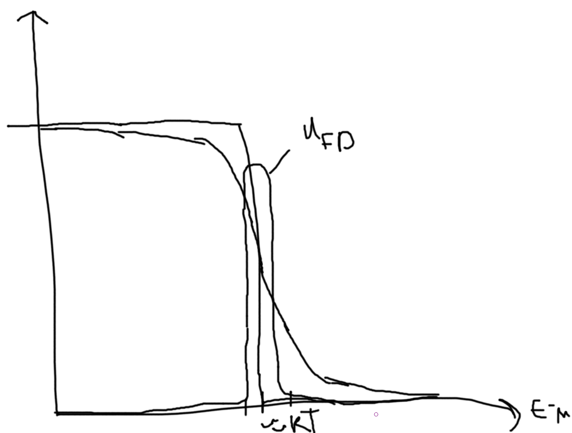
So, for MB this looks like a decaying exponential when plotted as a function of \(E-\mu\). For BE, there is asymototic behavior at 0 but decays above the MB exponential as \(E-\mu\) increases. For FD, there it is half at zero and decays strictly below the MB exponeitial, at \(-\infty\) it goes to 1.
At the classical limit, these different statistics converge to each other.
For very small \(T\), the BE curve approaches a delta function at \(0\). Since BE bounds the others above, the others become zero across the positive domain. The FD curve becomes a step-down function from \(1\) to \(0\).
Plotting Behavior of E
The plots are shifted over by \(\mu\). It gets more complicated if \(\mu\) is a function of temperature. Thus, the plots shift a bit left of \(E=\mu\) for a fixed value of \(\mu\).
Classical Limits
\(\langle O\rangle = \sum_\alpha p_\alpha O_\alpha, p_\alpha = \frac{1}{Z}\exp(-\beta E_\alpha)\).
Quantum: \(\langle O\rangle = \sum_k n(E_k-\mu)O_k\). \(N = \langle N\rangle = \sum_k n(E_k-\mu)\to N(\mu) \to \mu\).
For Fermions at \(T=0\), \(N = \sum_k 1\to E_k^{max,occupied} = \mu\equiv E_F=\epsilon_F\), the Fermi energy.
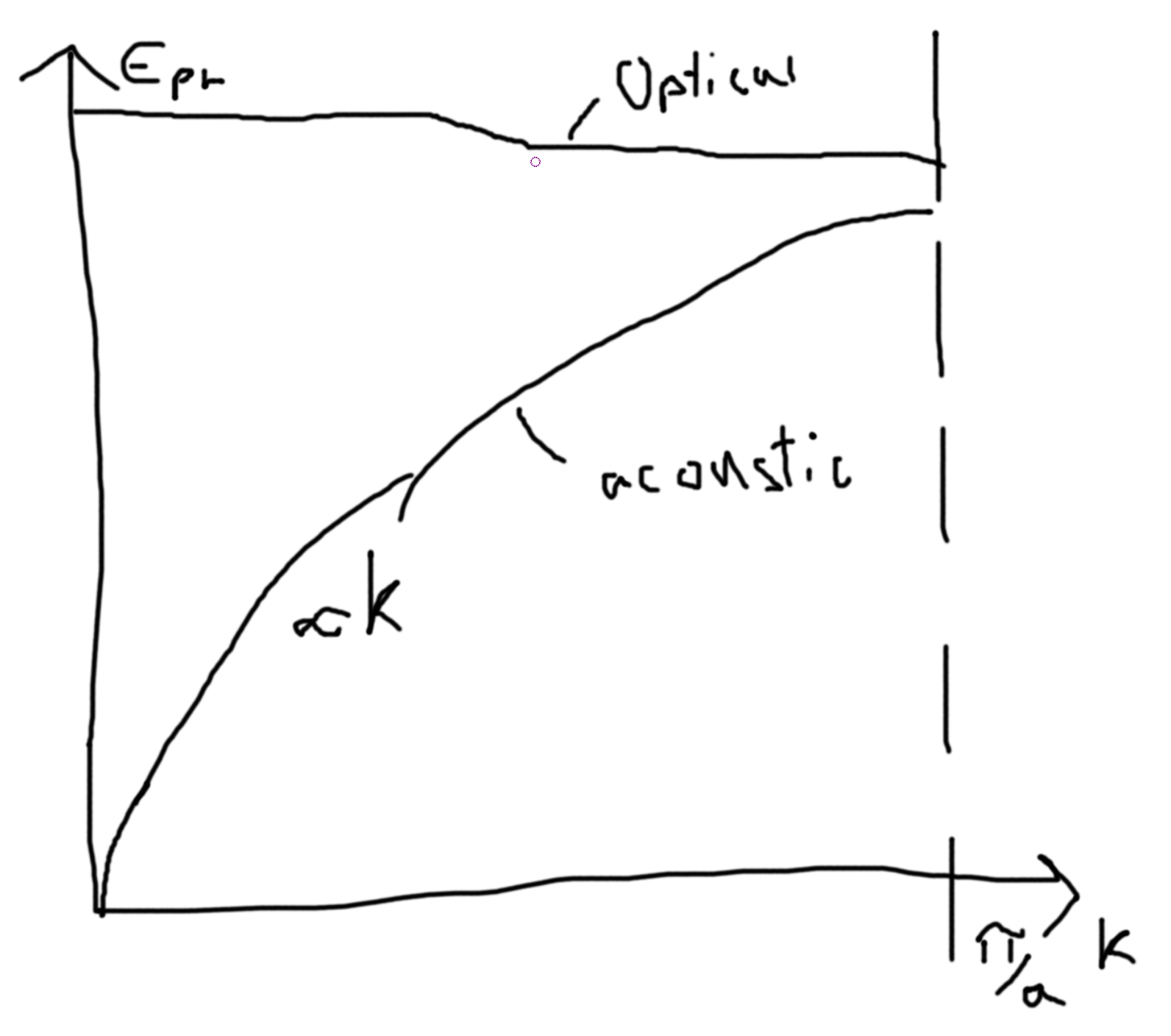
Einstein Gas: basic energy is \(\varepsilon = \hbar\omega\) the constant, and the linear model is \(\varepsilon=\hbar \gamma k\). These give the optical phonons which are the approximately the constant and the acoustic are approximately the linear.
\(\varepsilon(k) = \frac{\hbar^2k^2}{2m}\).
New Term
Review
- BE and FD statistics
- \(\langle n\rangle_{B/F} = \frac{1}{\exp(\beta(\epsilon-\mu))\mp1}\). Recall, if \(\epsilon=\mu\) then \(\langle n\rangle_F = \frac{1}{2}\) and \(\langle n\rangle_B \to\infty\).
Classical: \(\langle E\rangle = \sum_\alpha p_\alpha E_\alpha\), \(p_\alpha = \frac{\exp(-\beta E_\alpha)}{Z}\). For a classical system, \(Z = \frac{1}{N!}Z_1^N\). For a quantum system, we can compute \(\langle E_1\rangle\) to then get \(\langle E\rangle = N\langle E_1\rangle\). I.e. for a carbon atom, since the electrons are dependent we can describe it in the classical way, but if they were independent then we would need FD or BE.
\(\langle E\rangle = \sum_{\vec{k}} = n(\epsilon(\vec{k}),T,\mu(T))\epsilon(\vec{k})\). Need: \(\mu(T)\). For \(N\) quantum particles, we have \(N = N(\mu) = \sum_\alpha n_\alpha = \sum_{\vec{k}}n(\epsilon(\vec{k}),T,\mu(T))\). We can then invert this to get \(\mu(T)\).
QHO
We can solve this classically since we have just one particle (i.e. one oscillator). \(E_n = \left(n + \frac{1}{2}\right)\hbar\omega\). \(\langle E\rangle = -\frac{\partial\ln Z}{\partial\beta}\). \(Z = \sum_n \exp(-\beta E_n) = \exp(-\beta\hbar\omega/2)\frac{1}{1-\exp(-\beta\hbar\omega)}\). So, \(\langle E\rangle = \hbar\omega\left(\frac{1}{2} + \frac{1}{\exp(\beta\hbar\omega)-1}\right) = \left(\langle n\rangle+\frac{1}{2}\right)\hbar\omega\).
Density of States
\(N(,\mu,T) = \sum_k\langle n(\epsilon_k,\mu,T)\rangle\delta(\epsilon-\epsilon_k) = \int n(\epsilon(\vec{k}),\mu,T)g(\epsilon)d\epsilon\).
Particles in a Box
\(V = L^D\), for \(D-\) dimensions.
You can do this with:
- Standing Waves
\(\Psi\propto \sin\left(\frac{\pi}{L}n_xx\right)\), \(n\in\mathbb{Z}^+\). For the dimensions we have, each state takes up a volume of \(\left(\frac{L}{\pi}\right)^D\). Note, we only integrate over one quadrant, hence \(1/2^D\) of the total space \(\to \left(\frac{L}{2\pi}\right)^D\).
- Plane Waves (Periodic Boundary Conditions)
So, \(\Psi = \frac{1}{\sqrt{V}}\exp(i\vec{k}\cdot\vec{r})\). Our \(k\) is then, \(\frac{2\pi}{L}(n_x,n_y,n_z)^T\). Then, \(n_i\in\mathbb{Z} = \{0,\pm1,\pm2,\cdots\}\). For the dimensions we have, each state takes up a volume of \(\left(\frac{L}{2\pi}\right)^D\).
We need \(\epsilon(\vec{k})\).
- For massive fermions, \(\epsilon(\vec{k}) = \frac{\hbar^2k^2}{2m}\), from solving the Scrodinger Equation.
- For massive bosons, \(\epsilon(\vec{k}) = c\cdot\vec{p} = c\hbar|\vec{k}| = c\hbar k\).
If \(\epsilon(\vec{k})\propto f(|\vec{k}|)\). \(g(\epsilon)d\epsilon = 4\pi k^2\sum_{k_i}\left|\frac{dk_i}{d\epsilon}\right|^2d\epsilon \frac{V}{(2\pi)^3}g(k)\).
We use the simpler form, \(g(\epsilon)d\epsilon = 4\pi k^2\left|\frac{dk}{d\epsilon}\right|^2d\epsilon \frac{V}{(2\pi)^3}g(k)\) For (1), \(k^2 = \frac{2m\epsilon}{\hbar^2}\), \(\frac{dk}{d\epsilon} = \frac{1}{2}\sqrt{\frac{2m}{\hbar^2\epsilon}}\). Then, \(g(\epsilon)d\epsilon = \frac{V}{4\pi^2}\left(\frac{2m}{\hbar^2}\right)^{3/2}\sqrt{\epsilon}d\epsilon\).
Note, we could also write, \(g(\epsilon) = \frac{1}{V}\sum_{\vec{k}}\delta(\epsilon-\epsilon_{\vec{k}}) = \frac{1}{L^3}\frac{1}{\left(\frac{2\pi}{L}\right)^D}\int d\vec{k}\delta(\epsilon-\epsilon_{\vec{k}}) = \frac{1}{(2\pi)^D}\int d\vec{k}\delta(\epsilon-\epsilon_{\vec{k}}) = \begin{cases} 4\pi \int dk k^2 & D=3 \\ 2\pi\int dk k^1& D=2\\2\int dk k^0&D=1\end{cases}\). Then, \(k\to \epsilon\). \(d\epsilon = \left|\frac{d\epsilon}{dk}\right|dk\).
For phonons, \(g(k) = 2\), so it is typically not written.
Blackbody Radiation
\(\omega = ck\). \(c = \nu\cdot\lambda = \frac{\omega}{2\pi}\frac{2\pi}{k}\). \(\epsilon_{ph} = \hbar ck = \hbar\omega\).
Consider a box with a small hole in it. Put a photonic gas (Electromagnetic Radiation) in the box at a temperature \(T\).
\(g(\omega)d\omega = 2\frac{V}{(2\pi)^3}4\pi k^2\frac{dk}{d\omega}d\omega\) Note the leading two comes from \(g(k) = 2\) for the photonic gas. Then, \(k^2 = \frac{\omega^2}{c^2}\). \(\frac{dk}{d\omega}=\frac{1}{c}\).
Then, \(g(\omega)d\omega = \frac{V\omega^2}{\pi c^3}d\omega\).
The energy density is then, \(U(\omega)d\omega = V u(\omega)d\omega = \epsilon(\omega)g(\omega)n_{ph}(\omega,T)d\omega\). \(n_{ph}(\omega,T) = n_B(\mu=0)\).
\(U(\omega)d\omega = Vu(\omega)d\omega = \frac{\hbar\omega g(\omega)}{\exp(\beta\hbar\omega)-1}d\omega = \frac{V\hbar \omega^3}{\pi^2 c^3}\frac{1}{\exp(\beta\hbar\omega)-1}d\omega\). So, \(u(\omega) = \frac{\hbar \omega^3}{\pi^2 c^3}\frac{1}{\exp(\beta\hbar\omega)-1}\).
Aside
Remember that \(n_F = \frac{1}{\exp\left(\beta(\epsilon(k)-\mu)\right)-1}\).
Lecture 2
Consider that we have energy levels \(\epsilon_i\) for each particle. So, classically, \(\langle\epsilon\rangle = \sum p_n\epsilon_n\) and \(\langle E\rangle = N\langle\epsilon\rangle = \sum Np_n\epsilon_n = \sum n\epsilon_n\). Quantum mechanically, \(\langle\epsilon\rangle = \sum_k n^{FD/BE}(\epsilon_k,\mu,T)\epsilon_k\).
Remember for fermions, if there is a particle in \(\epsilon_1\) then there are no other particles in \(\epsilon_1\).
Other Boson Systems
Lattice vibrations in solids (phonons).
2 Models:
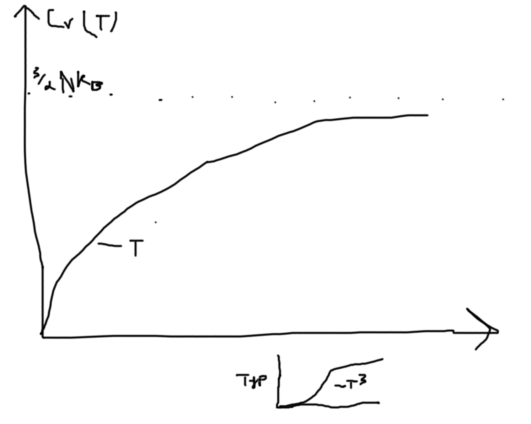
- Einstein model \(\epsilon_{ph} = \hbar\omega_0 = const\). We did this microcanonically in HW 641. \(U(T) = 3N_A\frac{\hbar\omega_0}{\exp\left(\frac{\hbar\omega}{kT}\right)-1}\). Low temp, \(C_V\propto\exp\left(-\frac{\hbar\omega_0}{kT}\right)\).
- Debye Model \(\omega(k) = v_Sk\). Where \(v_S = \frac{\partial \omega}{\partial k}\) is the speed of sound. That makes the acoustic curve linear. Has to fix \(N\) for the 3N modes. Find \(\omega_{max}\) from fixing \(N\) phonons which is \(3N_A\) times number of atoms. For low temperature, \(C_V(T)\propto T^3\) which is correct and Einstein’s model has the wrong prediction.
Fermions
They obey Fermi-Dirac statistics.
\(u_{FD} = \frac{1}{\exp(\beta(\epsilon-\mu))+1}; \epsilon(k) = \frac{\hbar^2k^2}{2m}\). The density of states is then \(g(\epsilon) = \frac{1}{4\pi^2}\left(\frac{2m}{\hbar^2}\right)^{3/2}\sqrt{\epsilon}\) and \(N = \int d\epsilon u_{FD}(\epsilon,\mu,T)g(\epsilon)\).
Can’t solve in general, so we do it in 3 stages.
- \(T=0\) (HW)
- High \(T\)
- Low \(T\)
For \(T=0\). \(u_{FD} = \Theta(x)\). \(\mu(T=0) = \epsilon_F\). So we want \(N = \int d\epsilon \Theta(\mu(T=0) - \epsilon)Vg(\epsilon)\). Then, \(=\int_0^{\epsilon_F}d\epsilon (2)\frac{V}{4\pi^2}\left(\frac{2m}{\hbar^2}\right)^{3/2}\sqrt{\epsilon}\). The two comes from spin 1/2. \(n = \frac{N}{V} = \cdots = \frac{1}{3\pi^2}\left(\frac{2m}{\hbar^2}\right)^{3/2}\epsilon_F^{3/2}\). Thus, \(\epsilon_F = \left(3\pi n\right)^{2/3}\frac{\hbar^2}{2m}\).
\(N = \sum_{\vec{k},\sigma} n_{FD}(T=0,\epsilon_{k}) = 2\frac{V}{(2\pi)^3}\int dk\Theta(\epsilon_F-\epsilon)\). \(\Theta(\epsilon_F-\epsilon)\to\Theta(k_F-k)\) from \(\epsilon_F = \frac{\hbar^2 k_F^2}{2m}\).
For high \(T\). Recall for an ideal gas: \(F = NkT\left(\ln\frac{N}{V}\lambda^3-1\right)\) eq [6.24]. \(\mu = \left.\frac{\partial F}{\partial N}\right|_{T,V} = \cdots = kT\ln(n\lambda^3)\). Then, for our case, \(u_{FD} = \frac{1}{\exp(\beta(\epsilon-\mu))+1}\to_{\mu < \epsilon} \exp(-\beta(\epsilon-\mu))\). So, \(N/V = n = \int d\epsilon \exp(-\beta(\epsilon-\mu))2\frac{1}{4\pi^2}\left(\frac{2m}{\hbar^2}\right)^{3/2}\sqrt{\epsilon} = \cdots = \left(\frac{2m}{\hbar}\right)^{3/2}\sqrt{\pi}(kT)^3\exp(\mu/kT)\). Solving this for \(\mu\) gives you \(\mu = kT\ln(n\lambda^3)\).
For low \(T\). So, \(kT\ll \epsilon_F\). The typical scale of \(\epsilon_F\) is roughly \(4-5 eV\). Note that \(1eV \sim 10000 K\).
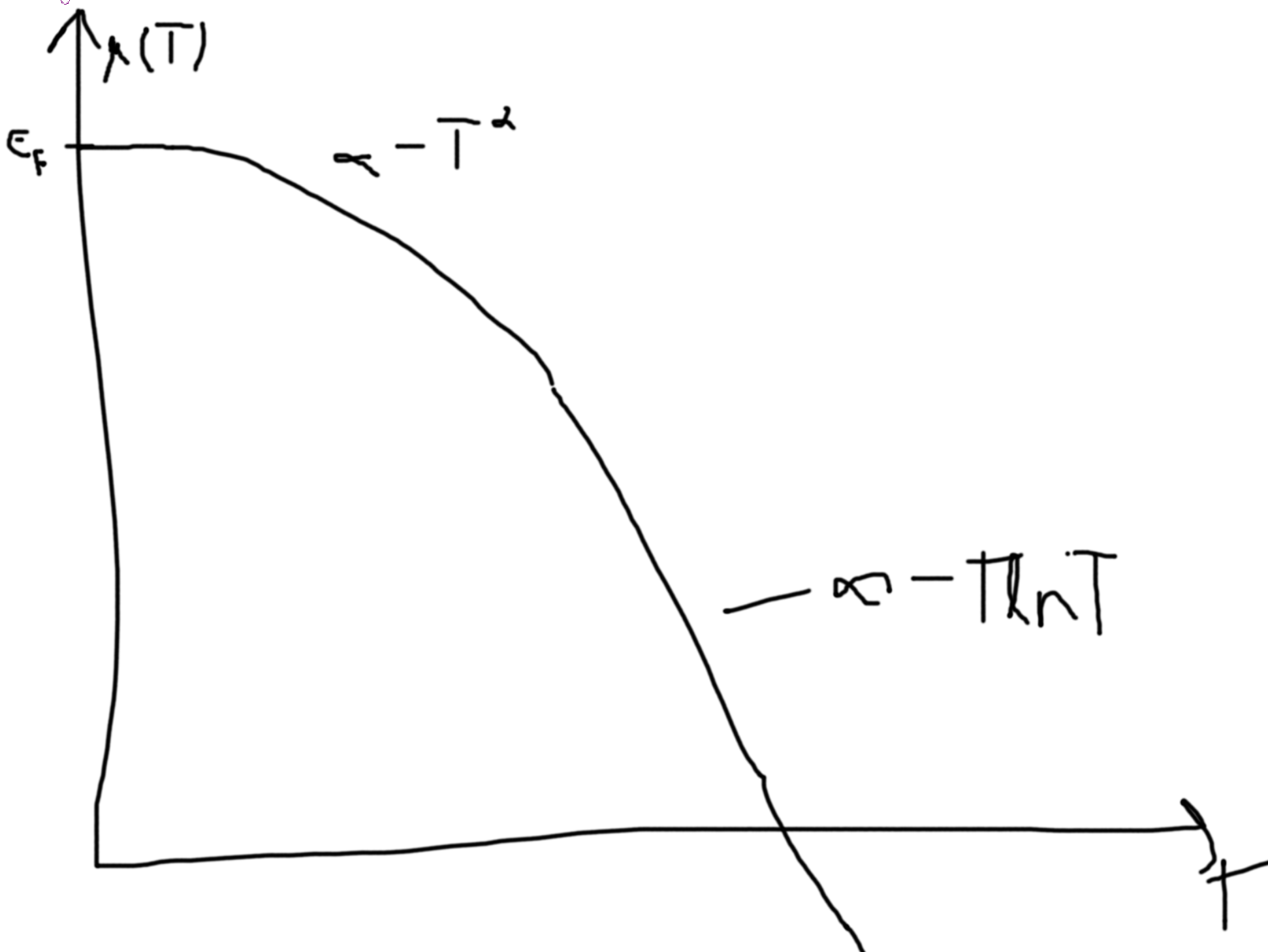
\(\frac{\phi}{V} = 2(-b(\mu)-\frac{\pi^2}{6}g(\mu)(kT)^2 + \mathcal{O}(kT)^4)\), \(b(\mu) = \int_{-\infty}^\mu d\epsilon a(\epsilon)\) and \(a(\epsilon) = \int_{-\infty}^\epsilon d\tilde{\epsilon}g(\tilde{\epsilon})\).
\(Z_G = \prod_k Z_{G_k} = \prod_k \left(1+\exp\left(-\frac{\epsilon_K-\mu}{kT}\right)\right)\), \(\phi = -kT\ln Z_G = -kT\sum_n\ln\left(1+\exp\left(-\frac{\epsilon_n-\mu}{kT}\right)\right)\to -kTV\int_{-\infty}^\infty d\epsilon g(\epsilon)\ln\left(1+\exp\left(-\frac{-\epsilon-\mu(T)}{kT}\right)\right)\) Invert \(N = N(\mu(T))\) to get \(\mu(T)\). Get \(N\) from \(N = -\left(\frac{\partial \phi}{\partial \mu}\right)_{V,T} = 2\left(\frac{\partial b}{\partial\mu} + \frac{\pi^2}{6}\frac{\partial g(\epsilon)}{\partial\epsilon}|_{\mu}(kT)^2\right)\). \(\frac{\partial b}{\partial\mu} = a(\mu) \approx a(\epsilon_F) + (\mu - \epsilon_F)\left(\frac{\partial a}{\partial\epsilon}\right)_{\epsilon_F} = \frac{N}{2} + (\mu-\epsilon_F)g(\epsilon_F)\). \(N = 2\left(\frac{1}{2}N + (\mu-\epsilon_F)g(\epsilon_F) + \frac{\pi^2}{6}\left(\frac{\partial g(\epsilon)}{\partial \epsilon}\right)_{\epsilon_F}(kT)^2\right)\). Thus, the second and third term must equal zero. So, \(\mu(T) = \epsilon_F - \frac{\pi^2}{6}\frac{1}{g(\epsilon_F)}\left(\frac{\partial g}{\partial \epsilon}\right)_{\epsilon_F}(kT)^2\)
 .
.
- Electrons are fermions with spin 1/2. \(2g_F = g_{e-}\)