Gibbs Phase Rules
\(n_w\): Number of ways to do work \(n_c\): Number of chemical +1: Heating/ cooling \(N = n_w + n_c + 1\) is the number of intensive parameters.
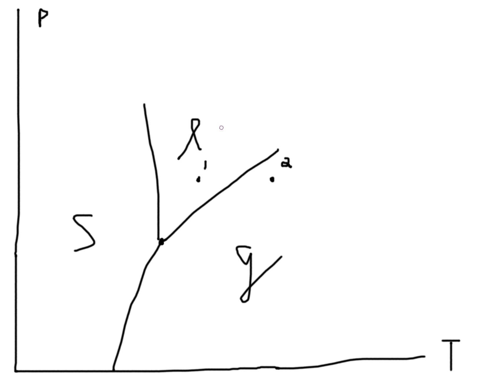
Constraints: If 2 phases coexist \(\mu_\ell = \mu_g\) is one constraint. If 3 phases coexist \(\mu_\ell = \mu_g\) and \(\mu_\ell=\mu_s\) gives 2 constraints. So, let \(p\) be the number of constraints. Then the degrees of freedom in our system is \(f = n_w + n_c + 1 - p\). Suppose we have 1 species \((n_c = 1)\) and 1 way of doing work (mechanical/ pressure for example) so \(f = 3 - p\). If we have 1 phase, \(p=1\) so \(f=2\) and so \(p(T)\) is an area. If we have 2 phases, \(p=2\) so \(f=1\) and so \(p(T)\) is a line. If we have 3 phases, \(p=3\) so \(f=1\) and so \(p(T)\) is a point (triple point).
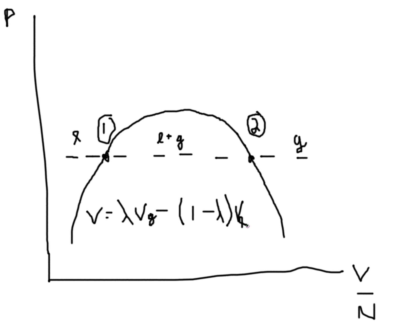
Say we fix \(N\), then we can plot \(P\) versus \(V/N\).
C.f. Suppose we have an alloy:
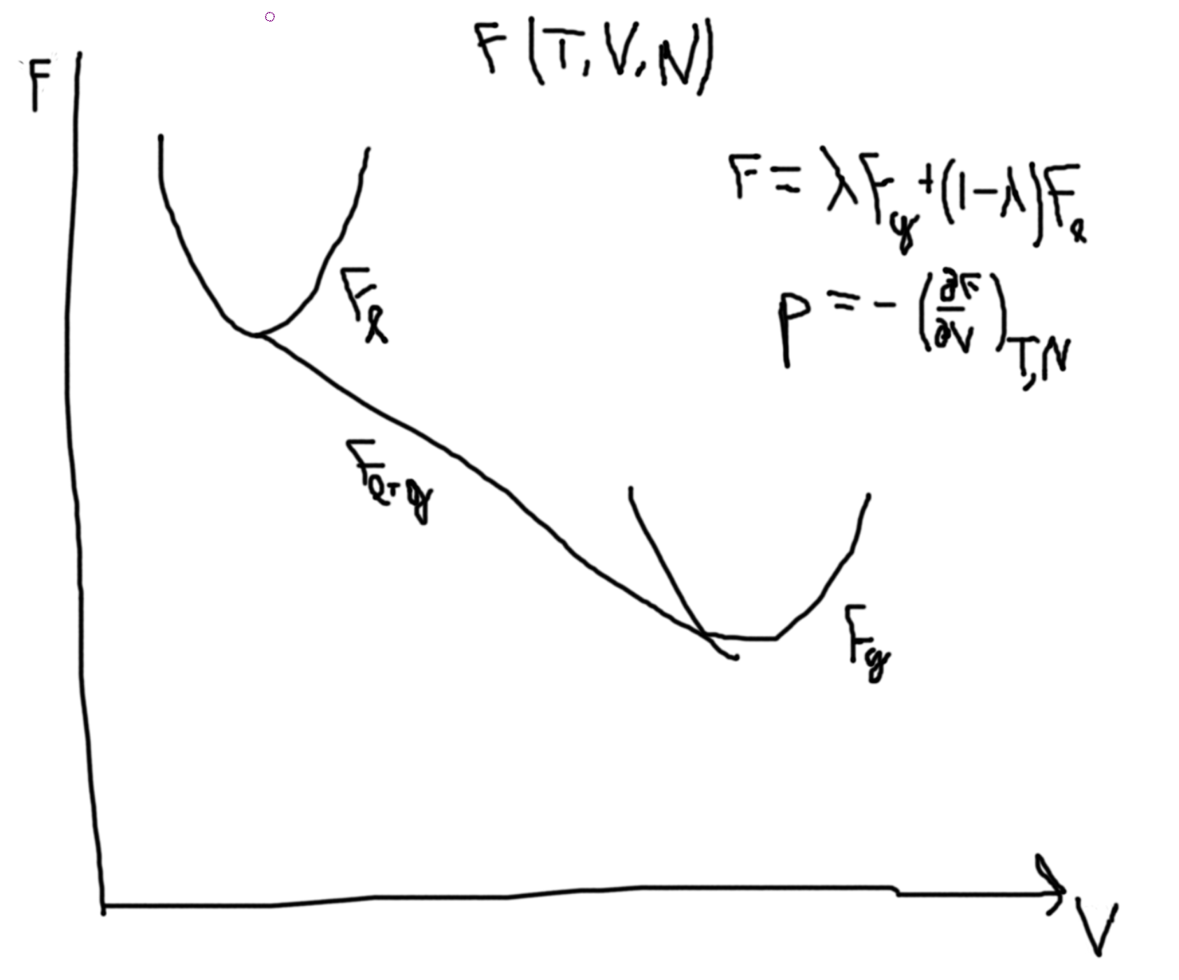
Suppose that we have a constant temperature \(\to G(T,p,N)\).
Then the Gibbs free energy of a liquid, we have a similar picture as \(F\) with \(T\) and \(N\). So, plotting \(G(p,T,N)\) versus temperature, we get two lines for liquids and gas that intersect at \(T_T\). The liquid line has a more gradual slope and a lower intercept. In the region before the \(T_T\) the gas line is called a supercooled gas and in the region after the liquid line (now above the gas line) is called a superheadted liquid.
So, \(G(T,p,N) = \mu N \Rightarrow \mu = \frac{G}{N}\). I.e. the chemical potential of liquid is less than that of a gas. \(S = -\left(\frac{\partial G}{\partial T}\right)_{P,N}\). \(\Delta S_{\ell-g} = \frac{Q}{T} = \frac{L N}{T}\) where \(L\) is the latent heat per particle. Hence, \(L = \frac{\Delta S \cdot T}{N}\). IMPORTANT To compute the latent heat you need to compute the entropy change. \(\Delta S =\) change in the slopes at the transition temperature.
Van der Waals Equation of State
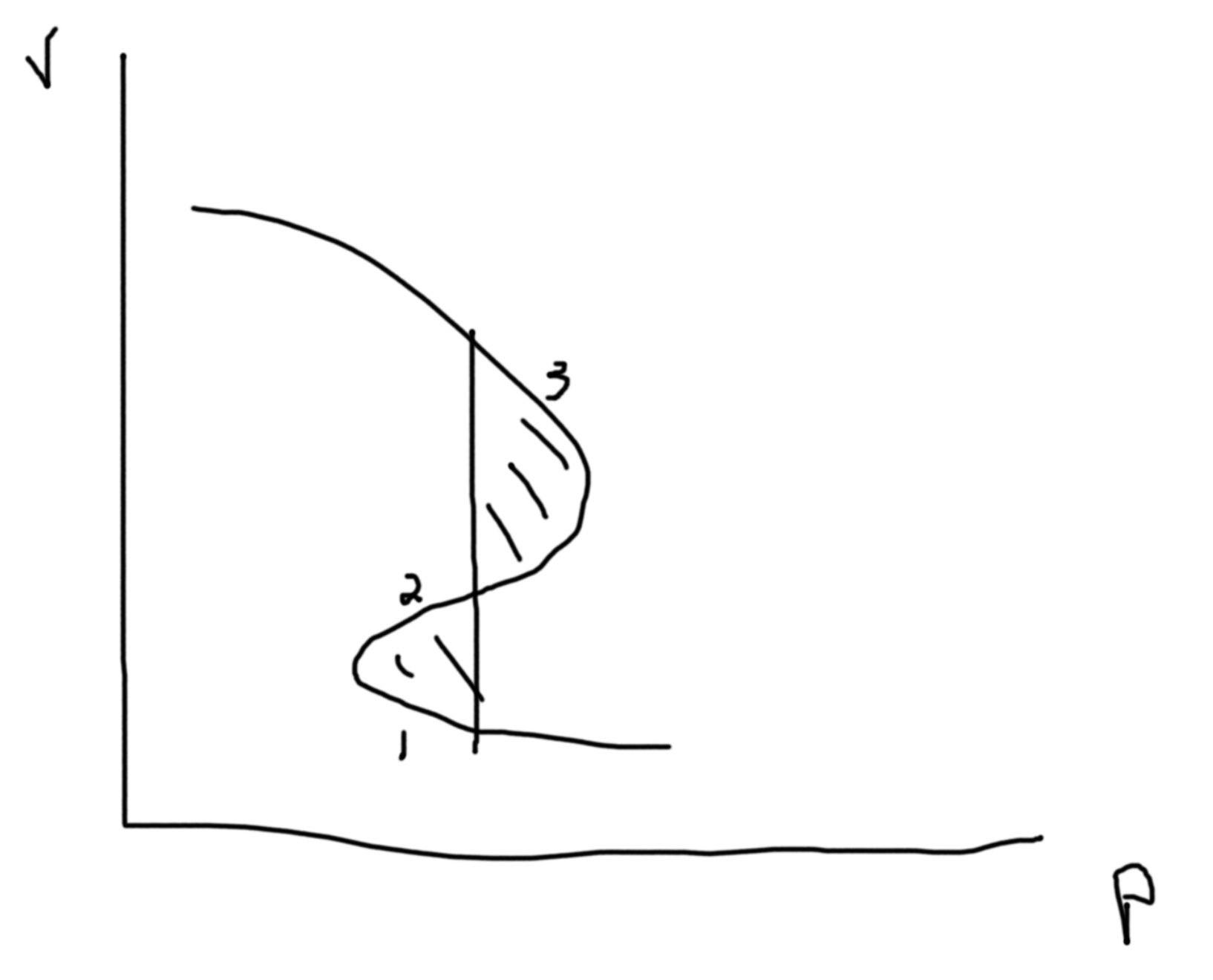
\(\left(p + a\frac{N^2}{V^2}\right)\left(V-Nb\right) = NkT\) \(a\) measures the attractive forces and \(b\) measures the volume taken up by each particle.
Recall analysis from previous homeworks. \(p(V)\propto V^\gamma\).
Stability conditions. For each conjugate pair you have (x, f) then \(\left(\frac{\partial x}{\partial f}\right)_{*}\geq 0\). Except, \(\alpha = \frac{1}{V}\frac{\partial V}{\partial T}\geq \text{or} \leq 0\). Compressibility gives condition for unstable states.
Between the two points we can draw a line at constant \(P\) such that area above equals area below. This denotes area of equal coexistence and so \(\mu_\ell=\mu_g\).
The dotted lines are unphysical regions.
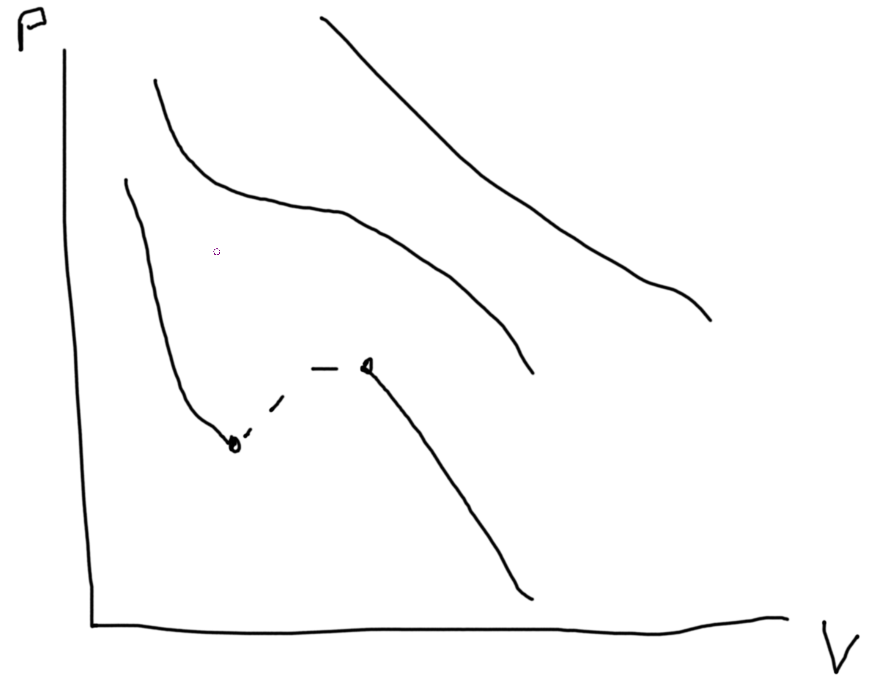 From \(p\leftrightarrow G\), \(dG = -SdT + Vdp + \mu dN\).
So \(\Delta G_{\ell-g} = \int_\ell^gdG = \int_{p_\ell}^{p_g}V(p)\).
From \(p\leftrightarrow G\), \(dG = -SdT + Vdp + \mu dN\).
So \(\Delta G_{\ell-g} = \int_\ell^gdG = \int_{p_\ell}^{p_g}V(p)\).
For a Reaction
\(3H_2+N_2 \rightleftharpoons 2NH_3\). In this setup, these could all be in a gaseous state. Assume this is the case. So \([H_2]^3[N_2]k_R(T) = \Gamma_R(T,p)\) and \(\Gamma_L(T) = k_L(T)[NH_3]^2\). Then, \(\frac{[NH_3]^2}{[H_2]^3[N_2]}=k_{eq}(T)\). This is the Law of mass action. Finding \(k_{eq}(T)\) we use the knowledge we are in gas phase and chemical potentials are equal.
Treat each constituent as an ideal gas. \(Z \to F \to \mu(T)\). \(\Delta F = \left(\frac{\partial F}{\partial N_{H_2}}\right)\Delta N_{H_2} + \left(\frac{\partial F}{\partial N_{N_2}}\right)\Delta N_{N_2} + \left(\frac{\partial F}{\partial N_{NH_3}}\right)\Delta N_{NH_3}\)
Considering the rightwards direction: \(\Delta F_R = -3\mu_{H_2} -\mu_{N_2} +2\mu_{NH_3}\). \(\Delta F_L = -\Delta F_R\).
\(F(T,V,N) = NkT\left(\ln \frac{N}{V}\lambda^3 - 1\right)+NF_0\) where the last term arises from the internal degrees of freedom of each of the \(N\) particles. So, \(\mu(T,V,N) = \left(\frac{\partial F}{\partial N}\right)_{T,V} = kT\left(\ln\frac{N}{V}\lambda^3-1\right)+NkT\frac{1}{N}+F_0 = kT\ln \frac{N}{V} + kT\ln\lambda^3 + F_0 = kT\ln \frac{N}{V} + \mathbb{C}(T) + F_0\). Inserting this in \(-3\mu_{H_2}-\mu_{N_2}+2\mu_{NH_{3}}=0\), we get \(-3\ln[H_2]-\ln[N_2]+2\ln[NH_3] = 2\mathbb{C}_{H_2}+\mathbb{C}_{N_2}-2\mathbb{C}_{NH_3} + 3F_{0,H_2} + F_{0,N_2} - 2F_{0,NH_3} = -\Delta F_{net}\). Then, \(\frac{[NH_3]^2}{[H_2]^3[N_2]} = k_{eq}(T) = k_0\exp\left(-\frac{\Delta F_{net}}{kT}\right)\). Recall, \(\Delta F = \Delta E-T\Delta S \approx \Delta E_{net}\) for solids and chemistry. Then, \(k_0 = \frac{\lambda_{H_2}^9\lambda_{N_2}^3}{\lambda_{NH_3}^6} = \frac{h^6 m_{NH_3}^3}{8\pi (k_BT)^3m_{H_2}^{9/2}m_{N_2}^{3/2}}\propto T^{-3}\).
Aside: C.f. with hydrogen atom, \(\frac{[p][e]}{[H]}=k(T)\) with \(n\cdot p=k(T)\).
Consider the one way reaction consisting of 5 particles, \(3H_2 + N_2\to NH_3\).
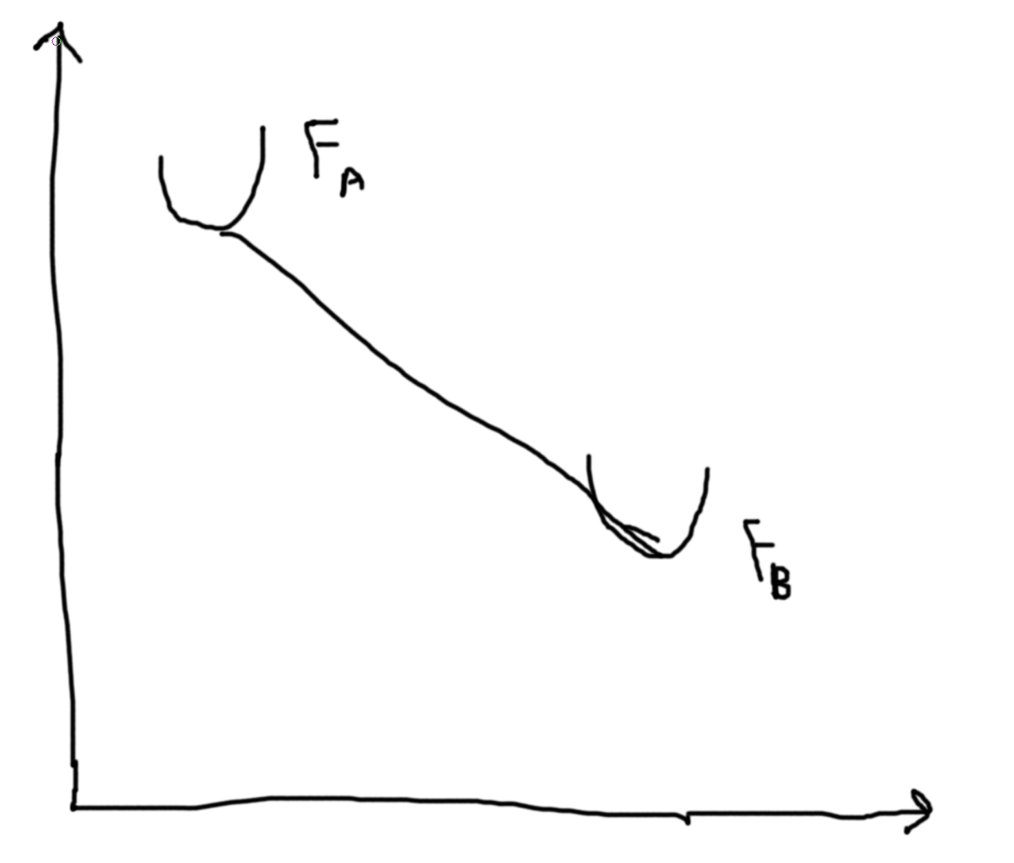
If we have \(M\) particles then we get a 3M dimensional space. Then we want to minimize energy in our 3M-1 dimensional space. Let \(X\) be the reaction coordinate. Let the y-axis be the energy.
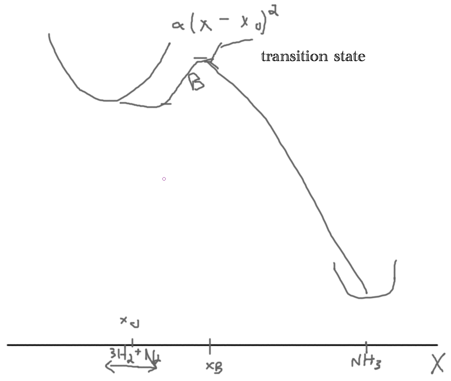 We argue that the rate is proportional to the Boltzman factor, \(\gamma \propto \exp\left(-\frac{B}{kT}\right)\), problem 6.11.
The assumptions are: no recrossing, reactions are in local equilibrium (in ’well’), equal distribution determines the number of particles crossing the well.
Let the probability distribution of the particles \(\rho(x)\). Then the probability distribution at the bottom of the well is \(\rho(x_0)\) and at the barrier \(\rho(x_b)\) such that \(\frac{\rho(x_b)}{\rho(x_0)} = \frac{\exp(-U(x_B)/kT)}{\exp(-U(x))/kT} = \exp(-B/kT)\).
Since \(B\gg kT\), most particles are near \(x_0\).
Then, \(U(x) = \frac{1}{2}M\omega^2(x-x_0)^2\).
So, \(\rho(x) = \sqrt{\frac{m\omega^2}{2\pi kT}}\exp\left(-\frac{m\omega^2}{2kT}(x-x_0)^2\right)\)
And so, \(\rho(x_0) = \sqrt{\frac{m\omega^2}{2\pi kT}}\).
We argue that the rate is proportional to the Boltzman factor, \(\gamma \propto \exp\left(-\frac{B}{kT}\right)\), problem 6.11.
The assumptions are: no recrossing, reactions are in local equilibrium (in ’well’), equal distribution determines the number of particles crossing the well.
Let the probability distribution of the particles \(\rho(x)\). Then the probability distribution at the bottom of the well is \(\rho(x_0)\) and at the barrier \(\rho(x_b)\) such that \(\frac{\rho(x_b)}{\rho(x_0)} = \frac{\exp(-U(x_B)/kT)}{\exp(-U(x))/kT} = \exp(-B/kT)\).
Since \(B\gg kT\), most particles are near \(x_0\).
Then, \(U(x) = \frac{1}{2}M\omega^2(x-x_0)^2\).
So, \(\rho(x) = \sqrt{\frac{m\omega^2}{2\pi kT}}\exp\left(-\frac{m\omega^2}{2kT}(x-x_0)^2\right)\)
And so, \(\rho(x_0) = \sqrt{\frac{m\omega^2}{2\pi kT}}\).
If the particle is \(\Delta x\) away from the top of the barrier with velocity \(v\) then \(\Delta x=v\Delta t\) gives the rate \(\Gamma_V=\rho(x_B)v\frac{\Delta t}{\Delta t} = \rho(x_b)v\). So, for all positive velocities, \(\Gamma = \int_0^\infty dv\Gamma_v\rho(v)\). Then, we are in equilibrium our velocities are normal distributed velocities, \(\rho(v) \propto \exp(-E_{kin}/kT) = \exp(-\frac{Mv^2}{kT})\) so \(\rho(v) = \sqrt{\frac{M}{2\pi kT}}\exp(-\frac{Mv^2}{2kT})\). Thus, \(\Gamma = \rho(x_B)\int_0^\infty v\rho(v)dv = \frac{\omega}{2\pi}\exp\left(-\frac{B}{kT}\right)\). Using multidimensional transition rate: \(\Gamma = \frac{\prod\limits_i\omega_i}{2\pi\prod\limits_j\omega_{j,B}}\exp\left(-\frac{B}{kT}\right)\). Where \(\omega_{j,B}\) denotes the saddle points.
If \(\omega\) is large we get a steep well.
Thus, in general it is difficult to analyze kinetic behaviors from equilibrium treatments.