Thermodynamics
Note: Intensive dExtensive
Hence,
\(dU=T\:dS + P\:dV + \mu\:dN\).
Extensive means \(f(aA, aB, aC) = af(A,B,C)\)
Definitions
Systems
Consists of many constituents (particles) \(N\gg 1\). Macroscopic.
We also wait long enough for the system it arrives to its thermodynamic (TD) equilibrium state.
If it is in the TD equilibrium state then it can be described by a few physical quantities called state variables.
Example of state variables: \(N,V,P,U,\mu,\tau,L,\sigma,A,T\). (3D: PV, 1D: $τ$L, 2D: $σ$A) All have physical meaning except temperature \(T\) which is defined in its relation to the others.
\(dW = \{\tau dx, \sigma dA, -pdV, \mu dN, B d\mu EdP\}\). We call the first term (p) the generalized force (intensive) and the second term (dV) the generalized displacement (extensive) and we call them both together conjugate pairs.
Temperature
Specifically, Temperature describes the process of energy exchange between different systems in thermal contact.
Energy flows (is transfered) from the system with high temperature to the system with low temperature.
The systems reach thermal equilibrium when no more net energy transfer takes place by heating or cooling and at this point their temperatures are equal.
Unit: [T] = K, Kelvin with \(T\gt 0\).
Boltzmann Constant
\(k_B = 1.38\cdot10^{-23}\frac{\text{J}}{\text{K}}\). So the units [\(k_bT\)]=[energy].
The equation of state (EOS) is a functional relationship between the state variables of a system (in TD equilibrium).
EOS can be obtained experimentally, ex. ideal gas law, \(pV=Nk_BT\) (dilute gas) which has a 200yr history.
Also can be obtained from first principles using SM or empirically (approximate). An example is the van der Walls EOS (vdW) \[ \left(p+a\frac{N^2}{V^2}\right)(V-Nb)=Nk_BT. \]
EOS are continuous and small changes in one variable lead to small changes in the other variables unless something dramatic happens (e.g. phase change, where the system fundamentally changes its state [symmetry change/ topology change]). This second part is the well behaved nature of the system. Example solid \(\leftrightarrow\) liquid. (Liquids are more fundamental since they have more symmetry [higher temperature generally implies more symmetries])
Small changes implies that you can linearize the EOS. An example from the ideal gas law: \(V\:dp + p\:dV=k_BT\:dN+Nk_B\:dT\). The \(dp,dV\) are called total differentials. vdW EOS describes both liquid and gas but has unphysical regions and requires interpretation.
Types of Equilibrium
- Thermal: \(T_A=T_B\)
- Mechanical: \(p_A=p_B\), \(\tau_A=\tau_B\)
- Chemical/ Diffusive: \(\mu_A=\mu_B\)
Process
A change of a system from one state (A) to another state (B).
Processes can be fast, slow, spontaneous, reversible, irreversible, quasistatic.
Quasistatic
A qs process is usually idealized process where all relevant state variables are well defined for the entire process.
In other words, a qs process is a sequence of TD equilibrium states.
Laws
Zeroth Law of TD
If A is in thermal equilibrium with C and B is in equilibrium with C then A is in thermal equilibrium with B.
First Law
Energy is conserved (provided we include energy changes by doing work and heating).
\(\Delta U = W + Q\) for Finite changes and always true.
\(dU = dQ + dW\) where d means small and \(dU\) is a total differential and this expression is always true.
Then, \(dU = dQ - pdV + \mu dN = TdS - pdV + \mu dN\)(\(dQ = TdS\) for Quasistatic Processes and is not always true).
Real Process \(\nrightarrow\) quasistatic (idealized) process.
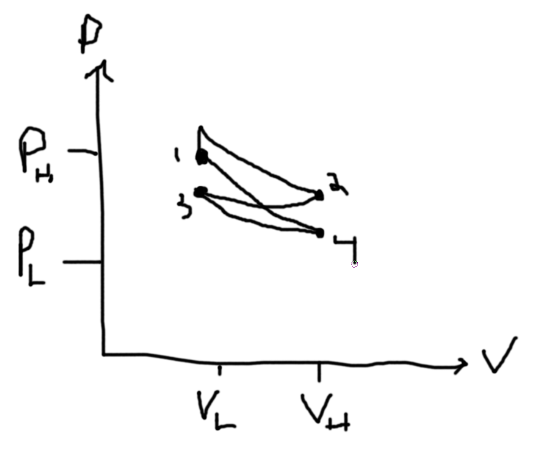
Example - Gasoline 4 stroke Engine
- Expand Volume (ignite and expand)
- Explosion
- Intake
- Compression
1–2 Q=0 3–4 Q=0 2–4 dV=0 3–1 dV=0
Ideal Gas
\(pV=NkT\), \(U \propto NkT\).
Processes
What is the sign of the entropy changes? V2 is initially empty.
- (A) Slow Expansion (environment has temperature T1 and gas is in piston environment with pressure P1 and volume V1 and gets expanded to 2V1 = V2)
- (B) Remove pin holding boundary between two volumes
- (C) Small Hole in Boundary between two volumes
- (D) Thermally insulated adiabatic wall (expand slowly)
- Questions to ask - Systemitize
- Is the process quasistatic? (A,D due to them being slow) (B is not due to it being fast) (C is not a sequence of equilibrium states and so it is not)
- Use First Law (ΔU = W + Q)
- Find initial and final states for (ΔU, W, Q)
- Find quasistatic process that have the same initial and final states to analysize the non-qs processes
For (A) there is no change in Energy. For (B) there is no Work. For (C) there is no Work. For (D) there is no Heat Exchange.
For A,B,C the final pressure is half, the final volume is double. Note that ABC has no change in internal energy. Q is zero. W = -Q for A and since work is done by the system, work is negative and so entropy increases. Because BC is not quasistatic (we cannot use dQ = TdS), we can relate them to A and see that entropy must increase. D has Q=0 and so entropy does not change but the temperature decreases since the internal energy decreases (from the fact that the system is doing work).
Systematize
- What are the state variables?
- How many (total)?
- How many are independent?
- Which ones are independent?
State Variables
1 energy, 2 state variables for heating, 2 variables for each work. Thus we have a total number of state variables is 1 + 2Nw + 2 state variables. And the number of independent state variables is Nw+1.
Assume we have amystery state variable X, we then assume U(X) so we can find the conjugate pair.
Relations between state variables are described by well behaved EOS (twice differentiated). I.e. small changes are equivalent to toal differentials.
Legendre? Transformation: Let Z=f(X,Y). \(dZ = \left.\frac{df}{dx}\right|_y\:dx+\left.\frac{df}{dy}\right|_x\:dy\). Let \(g(w,z)=f(x,y)\) then \(\left(\frac{\partial g}{\partial w}\right)_zdw + \left(\frac{\partial g}{\partial z}\right)_{w}dz = \left(\frac{\partial f}{\partial x}\right)_{y}dx + \left(\frac{\partial f}{\partial y}\right)_{x}dy\). I.e. convert \(U\) to \(F\) or \(H\), etc.
I.e. for the internal energy, \(dU = \left.\partial_S U\right|_{V,N}dS + \left.\partial_V U\right|_{S,N}dV + \left.\partial_N U\right|_{S,V}dN = TdS-pdV+\mu dN\). Note, that since we have $U(S,V,N) then we have \(T(S,V,N) = \frac{\partial U}{\partial S}\), i.e. a function of the same variables, and similarly for \(V,N\). Also, using this equivalence between the partial of the internal energy and the temperature, pressure, and chemical potential, we can then get \(S(T,V,N)\) and thus get \(U(T,V,N)\).
We can look at U(T,V,N). So, \(dU=\left.\frac{\partial U}{\partial T}\right|_{V,N}dT + \cdots dV + \cdots dN\). Note, that this is not necessarily equal to \(SdT - pdV + \mu dN\) since we are holding something different constant now. Thus, \(\frac{\partial U}{\partial V}_{T,N}\neq -p\) (at least not necessarily).
Consider: \(F=U-TS\). Then \(dF = dU - \left.\frac{\partial (TS)}{\partial T}\right|_{S,U}dS - \left.\frac{\partial (TS)}{\partial S}\right|_{T,U}dS = dU - SdT - TdS = TdS - pdV + \mu dN - SdT - SdT = -SdT -pdV + \mu dN\).
Energies
- U(S,V,N) (Assume: S(U,V,N), V(U, S, N), N(U, S, V), we may also write ℐ(U,S,V,N)=0)
- F = U - TS : F(T,V,N)
- H = U+PV : H(S,P,N)
- G = U - TS + PV : G(T,P,N)
- 𝓖 = U - TS - μN : 𝓖(T,P,μ)
Note from \(S(U,V,N)\) then \(dS = \frac{1}{T}dU + \frac{P}{T}dV-\frac{\mu}{T}dN\).
For Heating and Work
- Heating: S, T
- Work: (P,V), (μ, N), (B, μ), …
Notes
- Compressibility: \(\kappa_{S or T} = -\frac{1}{V}\left(\frac{\partial V}{\partial p}\right)_{S or T} \gt 0\) (we will show the greater than later)
- Thermal Expansion: \(\alpha = \frac{1}{V}\left(\frac{\partial V}{\partial T}\right)_{P}\) can be greater or less than zero.
- \(\frac{\partial Q}{\partial T}\) - Heat Capacity
Entropy Changes from Earlier Examples
Use an ideal gas. \(V_0\to V_1=2V_0\). Recall: \(U=cNkT\) and \(pV=NkT\).
Slow Isothermal Expansion
From slow, we know quasistatic. \(N,T,V\) Want: \(S\). \(dU = cNk\: dT\). Note, we have \(dU=TdS-pdV+\mu dN\). So, since this is isothermal, \(dU=0\). Then, \(TdS=pdV\). Then, \(\int_{S_0}^{S_1} f(S)dS = \int_{V_0}^{V_1}g(V)dV\). So, \(dS=\frac{P}{T}dV = \frac{Nk}{V}dV\) Then, \(\Delta S=Nk\ln2\).
Adiabatic Expansion
Calculate work done. Note \(dQ=0\).
\(dU = C_v\:dT = -p\:dV\). \(dH = C_p\:dT = V\:dp\).
\(C_vT = NkT\ln(V)\) \(C_pT = NkT\ln(P)\) \(\frac{C_V}{C_p}=\frac{\ln(V)}{\ln(P)}=\gamma\). Thus, \(P^\gamma = V\).
So, \(dW=-p\:dV \Rightarrow W = -\int_{V}^{2V} p\:dV\).
Alternatively (in class): \(dU=-p\:dV=cNk\:dT\) Then, \(p\:dV+V\:dp=Nk\:dT\) (4) \(PV=NkT\) \(p\:dV+V\:dp = NK\:dT\) (from 4). \(p\:dV+V\:dp = -\frac{P}{c}\:dV\) \(f_1(p)\:dp=f_2(V)dV\).
\(pV^\nu=\mathbb{C}\), \(\nu=\frac{c+1}{c}\).
\(W=\int_{V}^{2V}-p\:dV\).
Efficiency
Example Problems
One
\(f=g^2+h^2+\ell^2\) \(\ell=\ln(h-g)+h^2\). Using these two EOS, find \(\left(\frac{\partial f}{\partial \ell}\right)_h\) \(\left(\frac{\partial f}{\partial h}\right)_\ell\).
Strategy:
- Find the function with the variables mentioned: \(f(h,\ell)\)
- Linearize, \(df=\partial_h f\:dh + \partial_\ell f\:d\ell\).
Need \(f(h,\ell)\) since we have just those two variables. Then, we want: \(df = \left(\frac{\partial f}{\partial h}\right)_{\ell}dh = \left(\frac{\partial f}{\partial \ell}\right)_{h}d\ell\). We have: \(df = \left(\frac{\partial f}{\partial g}\right)_{h,\ell}dg + \left(\frac{\partial f}{\partial h}\right)_{g,\ell}dh = \left(\frac{\partial f}{\partial \ell}\right)_{h,g}d\ell\). \(d\ell = \left(\frac{\partial \ell}{\partial g}\right)_hdg + \left(\frac{\partial \ell}{\partial h}\right)_gdh\). Then, \(dg\) can be obtained from this expression of \(d\ell\). So, \(df = \left[\left(\frac{\partial f}{\partial h}\right)_{g,\ell}-\left(\frac{\partial f}{\partial g}\right)_{h,\ell}\frac{\left(\frac{\partial \ell}{\partial h}\right)_{g}}{\left(\frac{\partial \ell}{\partial g}\right)_h}\right]dh + \left[\left(\frac{df}{d\ell}\right)_{gh}+\frac{\left(\frac{\partial f}{\partial g}\right)_{h\ell}}{\left(\frac{\partial \ell}{\partial g}\right)_{h}}\right]d\ell\).
So, we need \(g(h,\ell)\). From the second EOS, \(g=h-\exp(\ell-h^2)\).
Two
Show \(\frac{U}{N}=f(T)\) independent of volume from ideal gas law \(pV=NkT\). I.e. show \(U\propto Nkf(T)\). If \(U(T,V)\) then \(dU=\partial_TU\:dT + \partial_VU\:dV\). So we must show \(\partial_V U=0\). Then, we have \(dU=T\:dS-p\:dV\). So, we have \(U(S,V)\) so we need \(S(T,V)\) to get \(U(T,V)\). Then, \(dS=\partial_T S\:dT + \partial_V S\:dV\). Hence, \(dU=T\partial_T S\:dT + T\partial_V S\:dV - p\:dV\). So, we must show \(T\partial_V S-p=0\). Now, we must find a Maxwell relation. We have \(V,T\). We have \(U(S,V,N)\), \(F(T,V,N)\), and \(H(S,p,N)\). So we use the free energy \(F\). This gives us, \(dF=-SdT-pdV\). \(\partial_V S=-\partial_V\partial_T F = -\partial_T\partial_V F=\partial_T p\). Then, \(T\partial_T p-p=0\). So, \(T\frac{Nk}{V}-\frac{NkT}{V}=0\), we have achieved what we needed!
More Problems
Second Law
Entropy always increases or stays the same. I.e. Entropy never decreases. Implies an Entropy maximum principle. A closed system after removal of one or more internal constraints will relax to that Thermodynamic Equilibrium state with the highest entropy consistent with the removed constraints. \(\delta S\geq 0\) all variations are possible.
- Mechanical
Say we have a block on a series of shelves and then we remove some shelves, then the mass will end up at the next possible state (a lower still existing shelf).
- Perturbed
Lets say we have a closed system in two halves. If we perturb it then \(\delta S_1 = \frac{1}{T_1}\delta U_1 + \frac{p_1}{T_1}\delta V_1 - \frac{\mu_1}{T_1}\delta N_1\), \(\delta S_2 = \frac{1}{T_2}\delta U_2 + \frac{p_2}{T_2}\delta V_2 - \frac{\mu_2}{T_2}\delta N_2\). Since it is closed: \(\delta U=\delta U_1+\delta U_2 = 0\), \(\delta V = \delta V_1 + \delta V_2 = 0\), \(\delta N = \delta N_2 + \delta N_2 = 0\). Then, redefine these such that \(\delta U = \delta U_1 = -\delta U_2\) etc. Then, \(\delta S = \delta S_1 + \delta S_2 = \left(\frac{1}{T_1}-\frac{1}{T_2}\right)\delta U + \left(\frac{p_1}{T_1}-\frac{p_2}{T_2}\right)\delta V - \left(\frac{\mu_1}{T_1}-\frac{\mu_2}{T_2}\right)\delta N = 0\), since \(S\) is maximum. Then, each coefficient must be zero. Thus, \(T_1=T_2\), \(p_1=p_2\), and \(\mu_1=\mu_2\).
- More General System - Equilibrium States from Helmholtz Free Energy
Let there be a system at \(V,T\) in an environment of temperature \(T\). Since \(\delta S\geq 0\) so \(\delta S_{sys} + \delta S_{env} \geq 0\).
\(dS_{sys} + dS_{env} \geq 0\). Multiplying by \(-T\), we get \(-T\:dS_{sys}-T\:dS_{env}\leq 0\), let this be (1). Also, \(dU = dU_{sys} + dU_{env} = 0\), let this be (2). Adding (1) and (2), \(dU_{sys}-T\:dS_{sys} + dU_{env} - T\:dS_{env}\leq 0\). Since the temperature is constant, \(-S_{sys}\:dT = 0\). \(dU_{sys}-T\:dS_{sys}-S_{sys}\:dT + dU_{env} - T\:dS_{env}\leq 0\). Using the Helmholtz free energy, \(F_{env}=U_{env}-T_{env}S_{env}\Rightarrow dF_{env}=dU_{env}-T_{env}\:dS_{env}-S_{env}\:dT_{env}\). Then, \(dU_{env} = dQ_{env} + dW_{env} = dQ_{env}\) since \(V\) is constant.
Then, \((dU_{sys}-T\:dS_{sys}-S_{sys}\:dT) + (dU_{env} - T\:dS_{env})=dF_{sys} + 0\leq 0 \Rightarrow \delta F\leq 0\). Thus, the minimizing the Helmholtz free energy gives the equilibrium states for constant temperature and volume.
If we had constant pressure and temperature then the Gibbs free energy is used, \(\delta G \leq 0\).
For a mechanical system, \(\delta U\leq 0\).
\(\Delta F_{sys} = \Delta U_{sys} - T\Delta S_{sys} \leq W + Q - T\frac{Q}{T}\) so \(\Delta F_{sys}\leq W\). This inequality becomes an equality for quasistatic processes.
\(\Delta F_{sys}\) during relaxation is \(\Delta Q_{sys} = -\Delta Q_{env}\) so \(dU = T\:dS-p\:dV\). Since \(dV = 0\), so \(\Delta U_{sys} = \int TdS = Q_{sys} = Q\), \(\Delta U_{env} = -Q\) so that \(\Delta U_{sys} + \Delta U_{env} = 0\).
- Enthalpy
Consider \(H=U+pV\) so \(dH = dU + p\:dV + V\:dp = T\:dS+V\:dp\) so \(\Delta H=\int T\:dS=Q\), \(Q_{sys} = -Q_{env} = Q\). Thus, \(\Delta H_{sys} = -\Delta H_{env}\) for constant pressure and temperature.
- General
For constant pairs:
V,T p,T \(\delta F \leq 0\) \(\delta G\leq 0\) \(\sum\delta U_i=0\) \(\sum\delta H_i = 0\)
Stability Conditions
Small perturbations do not give large changes instead they give small changes.
Example
Mechanics Example (1D)
Let \(U(x)\) be a function of position. Thus, \(F=-\frac{\partial U}{\partial x}\). At equilibrium states, \(F=-\frac{\partial U}{\partial x}=0\).
At the global minimum, the state is called stable. At a local minumum the state is metastable. At a maximum, the equilibrium is unstable.
Stability is the second order condition, \(\frac{\partial^2 U}{\partial x^2} \gt 0\).
If we have more than a single coordinate, then \(\sum_{i,j}\frac{\partial^2 U}{\partial x_i\partial x_j}\delta x_i\delta x_j\gt 0\).
If we go to a generalized force \(j_i=\frac{\partial U}{\partial x_i}\) then we can make a perturbation in the generalized force \(\delta j_i = \delta\left(\frac{\partial U}{\partial x_i}\right) = \sum_j\frac{\partial U}{\partial x_j\partial x_i}\delta x_j\). This gives us the condition, \(\sum_i \delta j_i\delta x_i \gt 0\) where \(x_i\) is a generalized displacement. We then see that \(\delta T \delta S + \sum_i\delta j_i\delta x_i + \sum_\alpha \delta \mu_a\delta N_a\gt 0\). And so \(\delta T\delta S - \delta p\delta V + \delta \mu\delta N\gt 0\).
Euler Relation
Extensivity
\(U(S,V,N)\) with \(U,S,V,N\) are extensive. Mathematically, \(\lambda U(S,V,N) = U(\lambda S,\lambda V, \lambda N)\). This is also referenced as U is a homogeneous function of order 1. Then, \(\frac{\partial}{\partial\lambda}\) on both sides and then set \(\lambda = 1\).
\(U(S,V,N) = \frac{\partial}{\partial\lambda}U(\lambda S,\lambda V, \lambda N) = \frac{\partial \lambda S}{\partial \lambda}\frac{\partial U}{\partial \lambda S} + \cdots\)
From Before
\(\delta T\delta S + \delta j\delta x + \delta\mu\delta N\geq 0\)
How to use? Variations \(\delta T,\delta x\) and, \(\delta N=0\).
\(\delta S(\delta T,\delta x), \delta J(\delta T,\delta x)\).
\(\delta S = \left(\frac{\partial S}{\partial T}\right)_x\delta T + \left(\frac{\partial S}{\partial x}\right)_T\delta x\) \(\delta j = \left(\frac{\partial j}{\partial T}\right)_x\delta T + \left(\frac{\partial j}{\partial x}\right)_T\delta x\)
From the original inequality, \(\left(\frac{\partial S}{\partial T}\right)_x(\delta T)^2 + \left(\frac{\partial S}{\partial x}\right)_T\delta x\delta T + \left(\frac{\partial j}{\partial x}\right)_T(\delta x)^2 + \left(\frac{\partial j}{\partial T}\right)_x\delta T\delta x\geq 0\).
Helmholtz: \(F(T,V), dF=-SdT-pdV\).
Consider the Maxwell relations from the Helmholtz free energy, \(dF=-S\:dT+j\:dx\) \(\frac{\partial^2 F}{\partial T\partial X}\Rightarrow \left(\frac{\partial S}{\partial x}\right)_T = -\left(\frac{\partial j}{\partial T}\right)_x\).
So, \(\left(\frac{\partial S}{\partial T}\right)_x(\delta T)^2 + \left(\frac{\partial j}{\partial x}\right)_T(\delta x)^2 \geq 0\).
Then, \(\delta x=0\) implies that \(\left(\frac{\partial S}{\partial T}\right)_x=\frac{C_x}{T}\geq 0\). Therefore, the constant volume/ length heat capacity must be non-negative.
Or, \(\delta T=0\) implies that \(\left(\frac{\partial j}{\partial x}\right)_T\geq0\Rightarrow \kappa_T=-\frac{1}{V}\left(\frac{\partial V}{\partial p}\right)_T\geq 0\). Therefore the constant temperature heat capacity must be non-negative.
If you have multiple particles, terms will appear in a similar fashion, and you will always have the \((\delta T)^2\) term. Specifically, if you have more than 1 \(J_i,x_i\) and include \(S,T\) in list of \((J_i,x_i)\). Then, the coefficients\(\cdot\left(\frac{\partial J_i}{\partial x_j}\right)_{i\neq j}\). The matrix of coefficients must be positive definite. This implies that all eigenvalues are positive and all subdeterminants are positive.
Example: \((p,-V), (\mu, N)\) at a constant \(T,N\), \(\begin{pmatrix} -\left(\frac{\partial p}{\partial V}\right)_{T,N} & \left(\frac{\partial p}{\partial N}\right)_{T,V} \ -\left(\frac{\partial \mu}{\partial V}\right)_{T,N} & -\left(\frac{\partial \mu}{\partial T}\right)_{T,V} \end{pmatrix}\)
\(\kappa_{T,N}=-\frac{1}{V}\left(\frac{\partial V}{\partial P}\right){T,N}\gt 0\). \(\left(\frac{\partial N}{\partial \mu}\right)_{T,V}\gt 0\). \(-\left(\frac{\partial p}{\partial V}\right)_{T,N}\left(\frac{\partial \mu}{\partial N}\right)_{T,V}+\left(\frac{\partial p}{\partial N}\right)_{T,V}\left(\frac{\partial \mu}{\partial V}\right)_{T,N}\gt 0\).
Consider \(G(p,T) = U-TS+pV\), take \(N\) to be constant and consider \(T_0,p_0\) fixed by environment. So, \(G(p,T)=U-T_0S+p_0V\). Then, \(\delta G(\delta S, \delta V) = \left(\frac{\partial G}{\partial S}\right)_V\delta V + \left(\frac{\partial G}{\partial V}\right)_S\delta V + \frac{1}{2}\left(\frac{\partial^2 G}{\partial S^2}\right)_V(\delta S)^2 + \frac{1}{2}\left(\frac{\partial^2 G}{\partial V^2}\right)_S(\delta V)^2 + \frac{\partial^2 G}{\partial S\partial V}\delta S\delta V = \left[\left(\frac{\partial U}{\partial S}\right)_V-T_0\right]\delta S + \left[\left(\frac{\partial U}{\partial V}\right)_S+p_0\right]\delta V + \left(\frac{\partial^2 U}{\partial S^2}\right)_V(\delta S)^2 + 2 \left(\frac{\partial^2 U}{\partial S\partial V}\right)\delta S\delta V + \left(\frac{\partial^2 U}{\partial V^2}\right)_S (\delta V)^2 \gt 0\). If \(\delta S, \delta V\) are independent then.
For \(\delta V=0\), \(\left(\frac{\partial^2 U}{\partial S^2}\right)_V=\left(\frac{\partial T}{\partial S}\right)_V=\frac{T}{C_V}\gt 0\). For \(\delta S=0\), \(\left(\frac{\partial^2 U}{\partial V^2}\right)_S=\frac{1}{V\kappa_S}=-\frac{V}{V}\left(\frac{\partial p}{\partial V}\right)_S\gt 0\).
Analyzing like a quadratic form, \(ax^2-f2bx;x_2+cx_2^2-\gt 0\), \(\overline{x}^T A\overline{a}+b^T\overline{x}\geq 1\). \(A=\begin{pmatrix} a & b \ c & d \end{pmatrix}\).
So, \(\left(\frac{\partial^2 U}{\partial S^2}\right)_V\left(\frac{\partial^2 U}{\partial V^2}\right)_S-\left(\frac{\partial^2 U}{\partial S\partial V}\right)\gt 0\) so \(\frac{1}{V\kappa_S C_V}\gt\left(\frac{\partial T}{\partial V}\right)_S^2\).
Example:
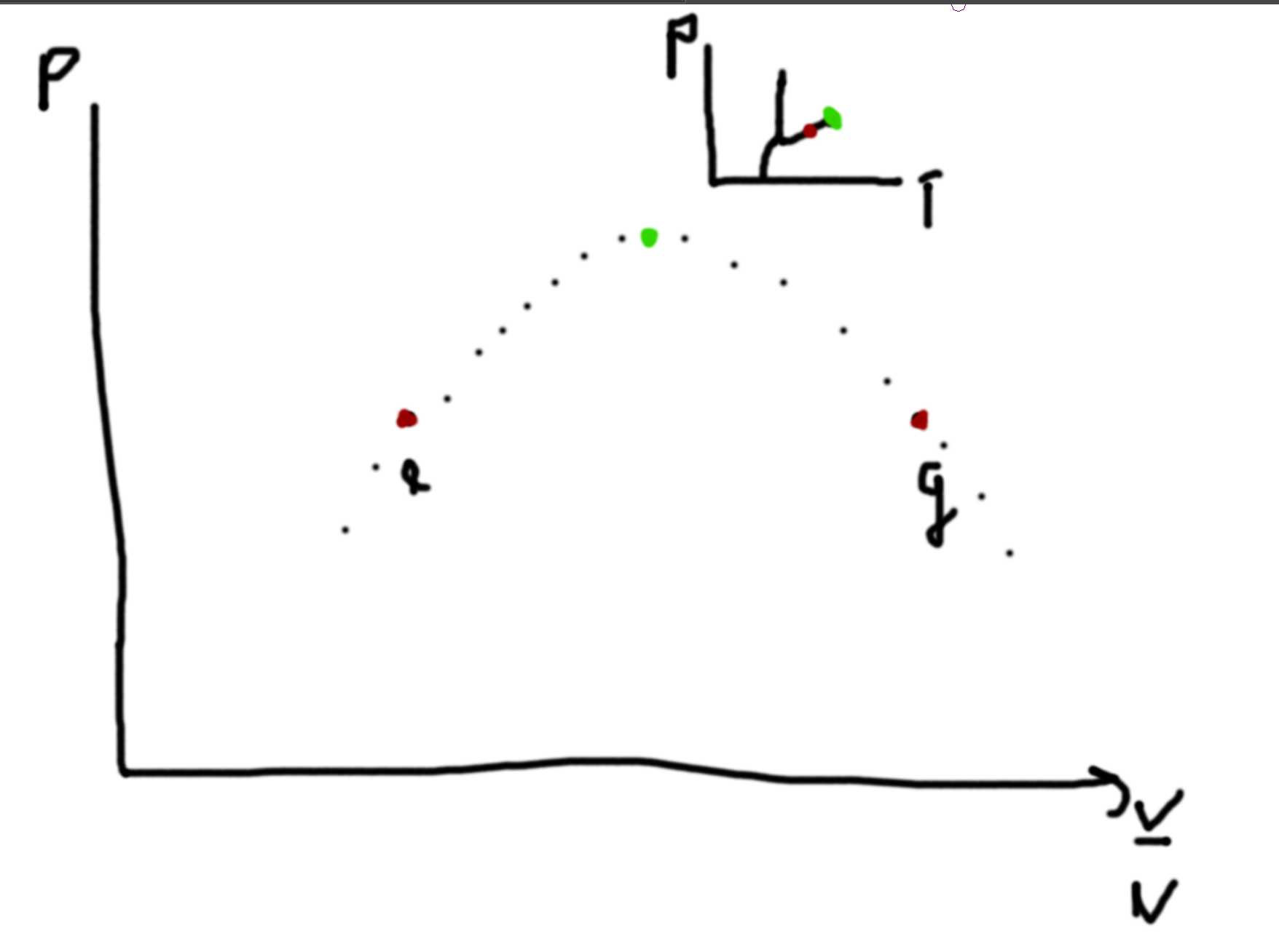
Consider a simple substance (one chemical composition) observe 3 phases, \((s,\ell,g)\).
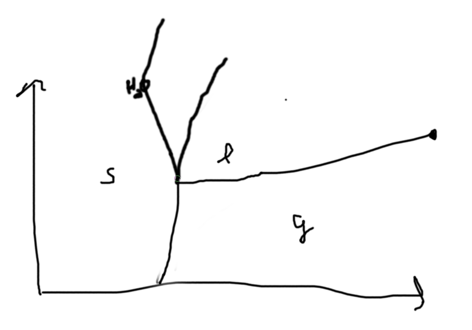
On the lines, we have coexistence of the phases, at intersections we have coexistence of all the phases. Phase boundaries.