Method of Images (Uniqueness Theorem)
Try to find external charges that give rise to the boundary conditions.
Example
Charged plate
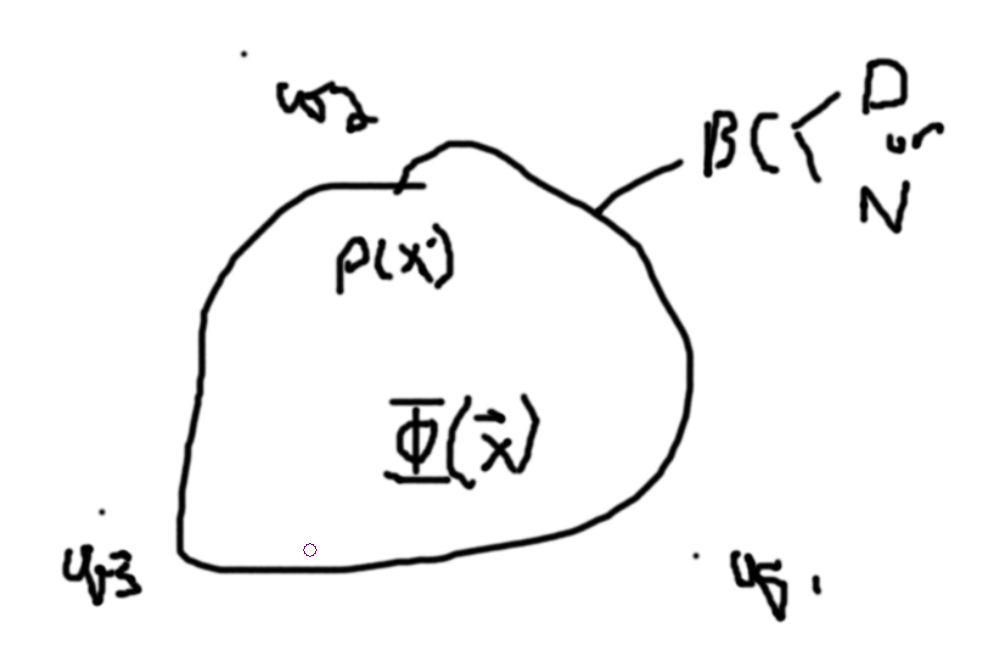
Let on right side of the charged plate (say it is a conductor to - infinity) have zero potential. Consider a charge \(q>0\) a distance \(d\) from the plate. The surface of the plate must have some surface charge induced from the point charge. Want to find \(\Phi(\vec{x}) = \Phi_q + \Phi_\sigma\) the total potential. Call this system 1.
Let this next system be system 2. Consider if we place a charge \(-q\) a distance \(d\) (along $z$-axis in cylindrical coordinates) from the plate on the other side. At the surface, we want to make sure we have a zero potential. Due to the symmetry, this is satisfied. We get a potential of \(\Phi(\vec{x}) = \frac{q}{4\pi\varepsilon_0 \sqrt{(z-a)^2+r^2}} - \frac{q}{4\pi\varepsilon_0 \sqrt{(z+a)^2+r^2}} = \frac{q}{4\pi\varepsilon_0}\left(\frac{1}{r_1}-\frac{1}{r_2}\right)\) using Cylindrical coordinates By uniqueness theorem, we find that \(\Phi_\sigma=\Phi_{-q}\). \(r_2 = \sqrt{R^2+a^2}\) with \(R^2=\sqrt{r^2+z^2}\) and \(r_1=\sqrt{R^2-a^2}\).
We can then use this to figure out the Electric field at the surface: \(E=\nabla \Phi\) and so \(\sigma(r) = \varepsilon_0 E_z(z=0)=-\varepsilon\left.\frac{\partial \Phi}{\partial z}\right|_{z=0}\) \(\frac{\partial\Phi}{\partial z} = \frac{q}{4\pi\varepsilon_0}\left(\frac{-1}{2}\frac{2(z-a)}{(r^2+(z-a)^2)^{3/2}}+\frac{1}{2}\frac{2(z+a)}{(r^2+(z+a)^2)^{3/2}}\right)\) which gives us \(\sigma(r) = \frac{-qa}{2\pi(r^2+a^2)^{3/2}}\).
Charge Near a Sphere
Let a charge \(q\) be placed near a grounded conducting sphere of radius \(a\) (outside at a distance \(d\)).
Consider if we place a charge \(q'\) a distance \(b\) towards \(q\) from the center of the sphere.
Then, due to no potential at the surface we get for \(z=+a\), \(\frac{q}{d-a}+\frac{q'}{a-b}=0\) and for \(z=-a\), \(\frac{q}{d+a}+\frac{q'}{a+b}\). Dividing these we get \(\frac{d+a}{d-a} = \frac{a+b}{a-b}\) then we get \(b=\frac{a^2}{d}\). We can then get \(q'=-\frac{a}{d}q\).
Conducting Sphere and Point Charge
Let \(q\) be placed ad distance \(d\) along the $z$-axis from the center of a grounded conducting sphere of radius \(a\). We want to find the potential outside of the sphere.
Ansatz: Using the method of images, we place a charge \(q' = -\frac{a}{d}q\) a distance \(b = \frac{a^2}{d}\) from the center of the sphere. So, the potential outside the sphere is: \(\Phi(x,y,z) = \frac{q}{4\pi\varepsilon_0}\left(\frac{1}{\sqrt{(z-d)^2+x^2+y^2}} - \frac{a}{d\sqrt{(z-b)^2+x^2+y^2}}\right) = \frac{q}{4\pi\varepsilon_0}\left(\frac{1}{\sqrt{(z-d)^2+x^2+y^2}} - \frac{a}{d\sqrt{\left(z-\frac{a^2}{d}\right)^2+x^2+y^2}}\right)\). In Spherical Coordinates: Let \(\vec{d}=d\hat{z}\), \(\vec{b}=b\hat{z}\), \(r_1^2=|\vec{x}-\vec{d}|^2 = (\vec{x}-\vec{d})\cdot(\vec{x}-\vec{d})\Rightarrow r_1=\sqrt{r^2+d^2-2dr\cos\theta}\), \(r_2^2=|\vec{x}-\vec{b}|^2 = (\vec{x}-\vec{b})\cdot(\vec{x}-\vec{b})\Rightarrow r_2=\sqrt{r^2+b^2-2br\cos\theta} =\sqrt{r^2+\frac{a^4}{d^2}-\frac{2a^2r}{d}\cos\theta}\). \(\Phi(r,\theta,\varphi) = \frac{q}{4\pi\varepsilon_0}\left(\frac{1}{\sqrt{r^2+d^2-2dr\cos\theta}} - \frac{a}{d\sqrt{r^2+\frac{a^4}{d^2}-\frac{2a^2r}{d}\cos\theta}}\right)\)
\(= \frac{q}{4\pi\varepsilon_0}\left(\frac{1}{\sqrt{r^2+d^2-2dr\cos\theta}} - \frac{1}{\sqrt{\left(\frac{rd}{a}\right)^2+a^2-2dr\cos\theta}}\right)\).
What if we let \(d=a+\delta\). Then, \(q'=-\frac{a}{d}q = -\frac{a}{a+\delta}q\approx -q\) and \(b = \frac{a^2}{d} = \frac{a^2}{a+\delta}\approx a-\delta\) from the binomial expansion of \(\left(1+\frac{\delta}{a}\right)^{-1}a \approx \left(1-\frac{\delta}{a}\right)a\).
Note, that the surface charge of the sphere is \(q'\) from Gausses law and the fact that \(\Phi_\sigma=\Phi_{q'}\) implies that \(\vec{E}_\sigma=\vec{E}_{q'}\).
Getting the surface charge density: \(\sigma = \varepsilon_0 E_n\). In our case, \(\sigma = \varepsilon_0 E_r\). Note, we only have \(\sigma=\sigma(\theta)\). Then, \(\sigma = \varepsilon E_r(r=a) = -\varepsilon_0\left.\frac{\partial \Phi}{\partial r}\right|_{r=a}=\cdots=-\frac{q}{4\pi}\left[-\frac{1}{2}\frac{2r-2d\cos\theta}{\sqrt{r^2+d^2-2dr\cos\theta}^3}+\frac{1}{2}\frac{2\frac{d^2}{a^2}r-2d\cos\theta}{\sqrt{\frac{d^2}{a^2}r^2+a^2-2dr\cos\theta}^3}\right]_{r=a} =-\frac{q}{4\pi}\left[-\frac{1}{2}\frac{2a-2d\cos\theta}{\sqrt{a^2+d^2-2da\cos\theta}^3}+\frac{1}{2}\frac{2\frac{d^2}{a^2}a-2d\cos\theta}{\sqrt{\frac{d^2}{a^2}a^2+a^2-2da\cos\theta}^3}\right] = \cdots =\frac{-q}{4\pi}\frac{\frac{d^2}{a}-a}{\sqrt{a^2+d^2-2ad\cos\theta}^3} =\sigma(\theta)\). Let \(\alpha = \frac{a}{d}\). Then, \(\sigma(\theta) = \frac{-q'}{4\pi a^2}\frac{(1-\alpha^2)}{\sqrt{1+\alpha^2-2\alpha\cos\theta}^3} = \sigma(\theta)=\sigma_0\frac{(1-\alpha^2)}{\sqrt{1+\alpha^2-2\alpha\cos\theta}}\). Note that \(\sigma_0\lt 0\) but everything else is positive so all charge on the surface is negative. Negative charge is more dense on the surface closest to the placed charge.
For \(\theta=0\), we get \(\sigma = \sigma_0\frac{1+\alpha}{(1-\alpha)^2}\). For \(\theta=\pi\), we get \(\sigma = \sigma_0\frac{1-\alpha}{(1+\alpha)^2}\).
\(\int\sigma(\theta)da = \pi\int_{-1}^1\sigma(\theta)\:a^2d\cos\theta = \pi\int_{-1}^1\frac{\sigma_0(1-\alpha^2)}{\sqrt{1+\alpha^2-2\alpha\cos\theta}^3}\:a^2d\cos\theta=\cdots =q'\).
Because the field and potentials are the same, the force felt by the charge due to the surface charge is the same as the force felt by the charge due to the mirror point charge. \(\vec{F}=q\vec{E}_\sigma\).
Non-Grounded Sphere
If we have a potential \(V\), then we can add a point charge \(q''\) at the center to get \(\Phi=V=V+0\) and completely solve the problem. I.e. \(V=\frac{1}{4\pi\varepsilon_0}\frac{q''}{a}\) implies \(q''=4\pi\varepsilon_0 aV\).
Known Initial Charge
If we know the charge on the sphere, then we can use this to figure out the potential at the surface. Note: \(Q=q''+q'\) from the previous one, so we can work backwards to get the mirror charge size (q’’). I.e. if we have \(Q=0\), then we can figure out that \(q''=q'\) and work from there.
- Using the Mirror Images to find the Dirchlet Green’s Function
Consider the case where we have a non-constant boundary, \(\Phi_s(r,\theta,\varphi)\) for some surface. For example let it be a sphere of radius \(a\). So, \(\Phi_s(a,\theta,\varphi)\). \(\rho=0\), \(\nabla^2\Phi=0\), \(\Phi(\vec{x})=-\frac{1}{4\pi}\int\left[\Phi_S\frac{\partial G}{\partial n'}\right]da'\)
Recall, \(G(\vec{x},\vec{x}')=G(\vec{x}',\vec{x})\), \(\nabla^2 G=-4\pi\delta(\vec{x}-\vec{x})\), \(G(\vec{x},\vec{x}')=\frac{1}{|\vec{x}-\vec{x}'|}+F(\vec{x},\vec{x}')\) with \(\nabla^2F=0\). \(G_D(\vec{x},\vec{x}')=0\) if \(\vec{x}\) or \(\vec{x}'\) is on the surface.
Then, the green’s function is just like a description of the potential at \(\vec{x}\) due to a point charge at \(\vec{x}'\). Thus, \(F(\vec{x},\vec{x}')\) is the potential due to the image charge. So for a chage placed at \(d\), \(G(\vec{x},\vec{x}')=\frac{1}{|\vec{x}-\vec{x}'}-\frac{\frac{a}{r'}}{|\vec{x}-\frac{a^2}{r'^2}\vec{x}'}\).
In our example, \(|\vec{x}-\vec{x'}|=\sqrt{r'^2+r^2-2rr'\cos\gamma}\) with \(\cos\gamma=\frac{\vec{x}\cdot\vec{x}'}{rr'} = \cos\varphi\sin\theta\cos\varphi'\sin\theta' + \sin\varphi\sin\theta\sin\varphi'\sin\theta + \cos\theta\cos\theta' = \cos\theta\cos\theta' + \sin\theta\sin\theta'\cos(\varphi-\varphi')\). \(\frac{r'}{a}\sqrt{r^2+\frac{a^4}{r'^2}-2r\frac{a^2}{r'}\cos\gamma}=\sqrt{\frac{r^2r'^2}{a^2}+a^2-2rr'\cos\gamma}\) Then, \(G(\vec{x},\vec{x}) = \frac{1}{\sqrt{r^2+r'^2-2rr'\cos\gamma}} - \frac{1}{\sqrt{\frac{r^2r'^2}{a^2}+a^2-2rr'\cos\gamma}}\)
\(\Phi(\vec{x}) = -\frac{1}{4\pi}\int_S\Phi_S\left(\frac{\partial G}{\partial n'}\right)da' = -\frac{1}{4\pi}\int_S\Phi_S\left(\frac{\partial G}{\partial r'}\right)a^2 d\Omega' = - \frac{a^2}{4\pi}\int_S\Phi_S\left(\frac{\partial G}{\partial r'}\right)d\Omega'\)
Note, if the region of interest is inside, then the surface normal points out. If the region of intrest is outside, then the surface normal points inside the surface.
So, if the region of interest is outside \(\Phi(\vec{x}) = \frac{a^2}{4\pi}\int_S\Phi_S\left(\frac{\partial G}{\partial r'}\right)d\Omega' = \frac{a^2}{4\pi}\int \Phi_S \left[\frac{-1}{2}\frac{2r-2r\cos\gamma}{\sqrt{r^2+a^2-2ra\cos\gamma}^3}+\frac{1}{2}\frac{2r^2/a-2r\cos\gamma}{\sqrt{r^2+a^2-2ar\cos\gamma}^3}\right]d\Omega = \frac{a^2}{4\pi}\int \Phi_S \left[\frac{-a^2+r^2}{a\sqrt{r^2+a^2-2ar\cos\gamma}^3}\right]d\Omega' = \frac{a(a^2-r^2)}{4\pi}\int \Phi_S \frac{-1}{\sqrt{r^2+a^2-2ar\cos\gamma}^3}d\Omega' = \frac{a(r^2-a^2)}{4\pi}\int_0^{2\pi}\int_{-1}^1\Phi(S)\frac{1}{\sqrt{r^2+a^2-2ar\cos\gamma}^3}\:d\cos\theta' d\varphi'\)
Consider when the surface is \(+V\) for positive \(z\) and \(-V\) for negative \(z\). I.e. \(\pm\theta/2\). Then, \(\Phi(\vec{x}) = \frac{a(r^2-a^2)V}{4\pi}\int_0^{2\pi}\left[\int_0^{\frac{\pi}{2}}-\int_{\frac{\pi}{2}}^\pi\right]d\cos\theta'd\varphi'\frac{1}{\sqrt{r^2+a^2-2ar\cos\gamma}^3}\) For \(\cos\theta'=t\), we get \(\cos\gamma=\cos\theta t+\sin\theta(\pm\sqrt{1-t^2})\sin\cos(\varphi'-\varphi)\)
For the second one, \(\vec{x}'\to-\vec{x}'\). Then, \(\cos\gamma=-\cos\gamma\) and \(\theta'\to\pi-\theta'\) and \(\varphi'\to\varphi+\pi\) and \(t\to-t\).
Thus, \(\Phi(r,\theta,\varphi)=\frac{Va(r^2-a^2)}{4\pi}\int_0^{2\pi}d\varphi'\int_0^1dt\left[\frac{1}{\sqrt{r^2+a^2-2ar\cos\gamma}^3}-\frac{1}{\sqrt{r^2+a^2+2ar\cos\gamma}^3}\right]\). What does the potential look on \(z-axis\), \(\Theta=0,\pi\).
For \(\Theta=0\), \(\cos\gamma\to\cos\theta' = t\) Then, \(\Phi(r,0,\varphi)=\frac{Va(r^2=a^2)}{2}\int_0^1dt\left[\frac{1}{\sqrt{r^2+a^2-2art}^3}-\frac{1}{\sqrt{r^2+a^2+2art}^3}\right]\).
\(\int_0^1\frac{1}{\sqrt{\alpha t+\beta}^3}dt = \frac{2}{\alpha}\left(\frac{1}{\sqrt{\beta}}-\frac{1}{\sqrt{\alpha+\beta}}\right) = \frac{2}{\alpha}\frac{\sqrt{\alpha+\beta}-\sqrt{\beta}}{\sqrt{\beta}\sqrt{\alpha+\beta}}\)
The potential is then, \(\Phi(z,0,\varphi) = V\left[1-\frac{z^2-a^2}{z\sqrt{z^2+a^2}}\right]\).
For a dipole: For \(r\gg a\) then \(\Phi(\vec{x})=\frac{1}{4\pi\varepsilon_0}\frac{\vec{p}\cdot\vec{x}}{r^3}\). Note that \(\vec{p}=q\vec{d}\) for the dipole. So, \(\frac{p}{4\pi\varepsilon_0}\frac{\cos\theta}{r^2}\).
For our system, let \(r\gg a\). Then, \(\sqrt{r^2+a^2-2ar\cos\gamma}^{-3}=\frac{1}{r^3}\sqrt{1+\frac{a^2}{r^2}-2\frac{a}{r}\cos\gamma}^{-3}\approx\frac{1}{r^3}\sqrt{1+\frac{3}{2}2\frac{a}{r}\cos\gamma}^{-3}\). For the largest order, \(=\frac{6}{r^3}\frac{a}{r}\cos\gamma\).
The other term gives \(\frac{1}{r^3}\sqrt{1-3\frac{a}{r}\cos\gamma}\).
So, \(\Phi(r,\theta,\varphi) = \frac{3Va^2}{2\pi r^2}\int_0^{2\pi}\int_0^1\left(\cos\theta\cos\theta' +\sin\theta\sin\theta'\cos(\varphi -\varphi')\right)\:d\Omega' = \frac{3Va^2\cos\theta}{ r^2}\).